A counter records the number of calls arriving at a switchboard in each of five one-minute intervals: \(3\) , \(5\) , \(2\) , \(4\) , \(6\) . If the counts are independent Poisson variables with mean \(\lambda\) , the probability of this exact record is
For \(\lambda=4\) this probability is about \(9.1\times10^{-5}\) ; for \(\lambda=2\) it is about \(1.9\times10^{-6}\) , almost fifty times smaller. Neither number is large, because any particular record of five counts is improbable. What is informative is the ratio. The data are fifty times more probable under \(\lambda=4\) than under \(\lambda=2\) , and it is hard to resist the conclusion that they support \(4\) over \(2\) .
Chapter 4 compared estimators that were handed to us. This chapter is about a method for producing them: regard the probability of the observed data as a function of the parameter, and estimate the parameter by the value at which that function is largest. The method is called maximum likelihood. It applies to any parametric model, respects sufficiency automatically, behaves sensibly under reparametrization, and, as Chapter 9 will show, is asymptotically as precise as any estimator can be in regular models. It also has failure modes, and most of them occur at the step that looks easiest, the maximisation.
5.1 The likelihood function
Definition 5.1 (likelihood and log-likelihood). Let the data \(X\) have density or mass function \(f(x;\theta)\) , and let \(x\) be the observed value. The likelihood function is the function of \(\theta\)
and the log-likelihood is \(\ell(\theta)=\log L(\theta)\) , with \(\ell(\theta)=-\infty\) where \(L(\theta)=0\) . For a random sample, \(L(\theta)=\prod_i f(x_i;\theta)\) and \(\ell(\theta)=\sum_i\log f(x_i;\theta)\) .
The formula is the one that defines the density. What changes is which argument is held fixed. As a function of \(x\) for fixed \(\theta\) it is a probability distribution and integrates to one. As a function of \(\theta\) for fixed \(x\) it is not a distribution at all: it need not integrate to one over \(\Theta\) , and the area under it has no meaning. Only ratios of its values at different parameters are interpreted.
Common mistake. Reading \(L(\theta)\) as the probability that the parameter equals \(\theta\) . It is the probability, or probability density, of the data computed under \(\theta\) . A statement of probability about the parameter requires a prior distribution and Bayes’ rule, the subject of Chapter 11.
Because only ratios matter, factors that do not involve \(\theta\) may be dropped, and two likelihood functions that are proportional carry the same message. By the factorization theorem, \(L(\theta;x)=g(T(x),\theta)h(x)\) for a sufficient statistic \(T\) , so the likelihood depends on the data, up to proportionality, only through \(T\) . Any procedure based on the likelihood function is automatically a function of the minimal sufficient statistic. The moment estimator \(2\bar X\) of Example 4.3 failed that test; nothing derived from the likelihood can.
Example 5.1: Reading a Poisson likelihood
For the five counts, with total \(20\) , the log-likelihood is, up to an additive constant,
Its derivative \(20/\lambda-5\) is zero at \(\lambda=4\) , positive for smaller \(\lambda\) , and negative for larger, so the likelihood has a single maximum at \(\hat\lambda=4=\bar x\) . Dividing by the maximum gives the relative likelihood
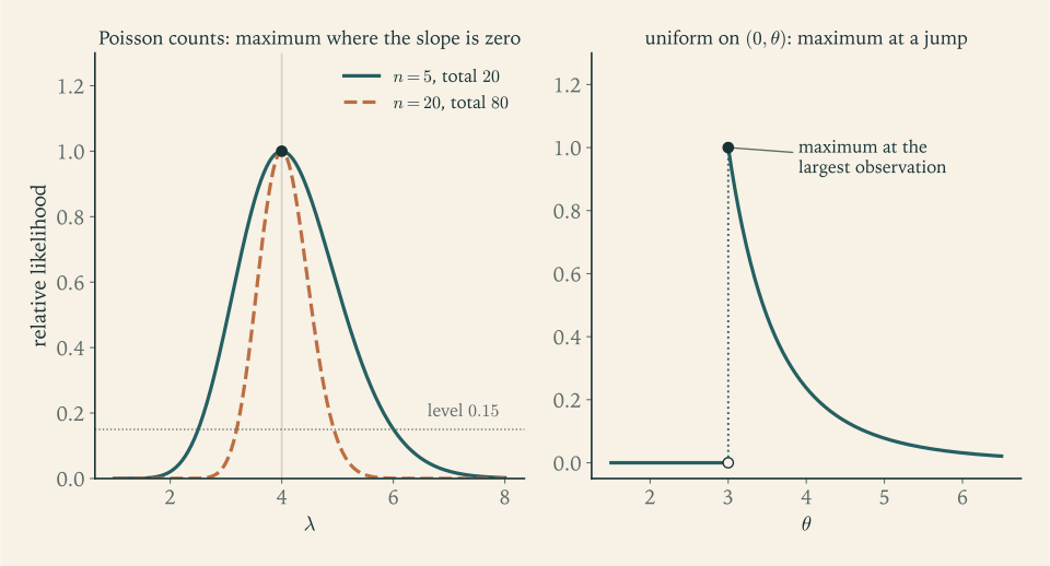
which measures how well each \(\lambda\) accounts for the data compared with the best-supported value. At \(\lambda=3\) it is about \(0.471\) and at \(\lambda=5\) about \(0.584\) ; these values are almost as well supported as \(4\) . At \(\lambda=2\) it is about \(0.021\) and at \(\lambda=6\) about \(0.151\) . The function is not symmetric about its maximum: it falls more steeply on the left. The set of \(\lambda\) with relative likelihood at least \(0.15\) is approximately the interval from \(2.50\) to \(6.00\) , a first, informal answer to “which values of \(\lambda\) are plausible?”
Had there been twenty counts with total \(80\) , the maximum would still be at \(4\) , and the relative likelihood \((\lambda/4)^{80}e^{-20(\lambda-4)}\) would be the fourth power of the previous one: the same shape, much narrower. The left panel of Figure 5.1 shows both. The sharpness of the peak is the visual form of precision, and Section 5.4 turns it into a number.
5.2 Maximum likelihood estimators and how to find them
Definition 5.2 (maximum likelihood estimator). A maximum likelihood estimate is a value \(\hat\theta=\hat\theta(x)\in\Theta\) with
The corresponding function of the data, \(\hat\theta(X)\) , is a maximum likelihood estimator, abbreviated MLE.
The definition is a global maximisation over the parameter space. Calculus enters only as a tool for carrying it out. When \(\ell\) is differentiable and \(\Theta\) is an open set, a maximiser must satisfy the likelihood equation \(\partial\ell/\partial\theta_j=0\) for each component, but the equation is necessary, not sufficient, and a complete solution has four steps: find the support of the model and write the likelihood with its indicators; solve the likelihood equation where the log-likelihood is differentiable; verify that a solution is a maximum, by a second-derivative test or by concavity; and compare with the boundary of \(\Theta\) and with points where differentiability fails.
Example 5.2: Both parameters of a normal sample
Nine measurements of a reference length, in millimetres, are
modelled as a random sample from \(N(\mu,\sigma^2)\) with \(\theta=(\mu,\sigma^2)\in\mathbb R\times(0,\infty)\) . Write \(v=\sigma^2\) . The log-likelihood is
The likelihood equations are
The first gives \(\hat\mu=\bar x\) and then the second gives \(\hat v=\frac1n\sum(x_i-\bar x)^2\) . For the data, \(\sum x_i=90.9\) , so \(\hat\mu=10.1\) , and \(\sum(x_i-\bar x)^2=0.74\) , so \(\hat\sigma^2=0.74/9\approx 0.0822\) and \(\hat\sigma\approx 0.287\) .
That this critical point is the global maximum can be seen without second derivatives. For any \(v\)
, the sum \(\sum(x_i-\mu)^2\)
is smallest at \(\mu=\bar x\)
, so \(\ell(\mu,v)\le\ell(\bar x,v)\)
. The function \(v\mapsto\ell(\bar x,v)=-\frac n2\log(2\pi v)-\frac{0.74}{2v}\)
tends to \(-\infty\)
as \(v\to0\)
and as \(v\to\infty\)
, and has the single critical point \(\hat v\)
, which is therefore its maximum. Alternatively, the second-derivative test for a function of two variables (math.multivariable-calculus.second-derivative-test) applies: at \((\hat\mu,\hat v)\)
the Hessian is diagonal with entries \(-n/\hat v\)
and \(-n/(2\hat v^2)\)
, both negative (Exercise 4).
The maximum likelihood estimator of the variance uses the divisor \(n\) , not \(n-1\) . It is the divisor-\(n\) estimator, the analogue for \(n=9\) of the middle row of the table in Example 4.1: biased, with smaller mean squared error than \(S^2=0.74/8=0.0925\) . Maximum likelihood does not aim at unbiasedness and does not in general deliver it.
Example 5.3: A maximum where no derivative vanishes
Let \(x_1,\dots,x_n\) be a random sample from the uniform distribution on the closed interval \([0,\theta]\) , with \(\theta>0\) . The likelihood is
It is zero for \(\theta\) below the largest observation, because such a \(\theta\) makes the data impossible. On \([x_{(n)},\infty)\) it equals \(\theta^{-n}\) , which is strictly decreasing. The maximum is therefore at the left end of that range: \(\hat\theta=x_{(n)}\) . For the data \(0.3\) , \(0.5\) , \(0.4\) , \(3.0\) , \(0.8\) of Example 4.3, \(\hat\theta=3.0\) , where the moment estimate was the impossible value \(2.0\) .
The derivative of \(\log L\) on the region where \(L\) is positive is \(-n/\theta\) , which is never zero. A solver that looks only for stationary points finds nothing. The maximum sits at a discontinuity, shown in the right panel of Figure 5.1. The lesson is general for models whose support depends on the parameter: write the indicator, and maximise by inspection.
Two further remarks. If the density is taken to be positive on the open interval \((0,\theta)\) instead, the likelihood is \(\theta^{-n}\mathbf 1\{\theta>x_{(n)}\}\) , whose supremum is approached as \(\theta\) decreases to \(x_{(n)}\) and is not attained; strictly speaking no MLE exists. Changing a density at a single point does not change the distribution, so one chooses the version for which the maximum is attained. And the estimator \(\hat\theta=X_{(n)}\) is biased, as Example 4.3 showed: the MLE always sits at or below the true endpoint.
Common mistake. Solving the likelihood equation and stopping. A root of the equation may be a minimum or a saddle, may be one of several local maxima, or may lie outside the parameter space; and the maximiser may be a boundary point or a point of discontinuity where the equation does not hold at all.
The parameter space matters as much as the formula. Suppose \(X_1,\dots,X_n\) are a random sample from \(N(\mu,1)\) and it is known that \(\mu\ge0\) . The log-likelihood is \(-\frac12\sum(x_i-\mu)^2\) up to a constant, a concave parabola in \(\mu\) with vertex at \(\bar x\) . If \(\bar x\ge0\) the vertex is in the parameter space and \(\hat\mu=\bar x\) . If \(\bar x<0\) the parabola is decreasing on \([0,\infty)\) and the maximum is at the boundary: \(\hat\mu=0\) . In one formula, \(\hat\mu=\max(\bar x,0)\) . Similarly, for \(n\) Bernoulli trials with no successes the log-likelihood \(n\log(1-p)\) is decreasing in \(p\) ; on the closed parameter space \([0,1]\) the MLE is \(\hat p=0\) , and on the open interval \((0,1)\) none exists.
A maximum likelihood estimate need not be unique either. In the uniform model on \((\theta,\theta+1)\) of Example 3.3 the likelihood equals \(1\) for every \(\theta\) in the interval from \(x_{(n)}-1\) to \(x_{(1)}\) and \(0\) elsewhere, so every point of that interval is an MLE.
For the exponential families of Section 3.4 none of these difficulties arises in the interior. In natural form the log-likelihood of a random sample is \(\ell(\eta)=\eta\sum T(x_i)-nA(\eta)\) plus a constant. Its derivative is \(\sum T(x_i)-nA'(\eta)\) and its second derivative is \(-nA''(\eta)\le0\) by Proposition 3.7. So \(\ell\) is concave, any solution of the likelihood equation is a global maximum, and the equation itself reads
that is, choose the parameter so that the expected value of the natural statistic equals its observed average. For exponential families maximum likelihood and the method of moments applied to the natural statistic coincide.
5.3 Invariance under reparametrization
Suppose the quantity of interest is not \(\lambda\) but the probability \(e^{-\lambda}\) that a minute passes with no calls. One could rewrite the model in terms of \(\eta=e^{-\lambda}\) and maximise again. The result is always the obvious one.
Theorem 5.3 (invariance of maximum likelihood). Let \(\hat\theta\) be a maximum likelihood estimate of \(\theta\) and let \(g\) be any function defined on \(\Theta\) . Define the induced likelihood of a value \(\eta\) in the range of \(g\) by
Then \(g(\hat\theta)\) maximises \(L^\ast\) .
Proof. The point \(\hat\theta\) belongs to the set over which the supremum defining \(L^\ast(g(\hat\theta))\) is taken, so \(L^\ast(g(\hat\theta))\ge L(\hat\theta)\) . For any other \(\eta\) , every \(\theta\) with \(g(\theta)=\eta\) satisfies \(L(\theta)\le L(\hat\theta)\) because \(\hat\theta\) is a global maximiser, so \(L^\ast(\eta)\le L(\hat\theta)\) . Combining, \(L^\ast(\eta)\le L^\ast(g(\hat\theta))\) for every \(\eta\) .
When \(g\) is one-to-one the induced likelihood is just the likelihood written in the new parameter, and the theorem says the MLE transforms like the parameter. When \(g\) is many-to-one, as with \(g(\mu,\sigma^2)=\mu/\sigma\) , the induced likelihood maximises over all parameter values sharing the same \(g\) , and the conclusion is the same. The MLE of \(g(\theta)\) is \(g(\hat\theta)\) .
Example 5.4: Derived quantities from two fitted models
Switchboard. With \(\hat\lambda=4\) , the MLE of the probability of a minute with no calls is \(e^{-4}\approx0.0183\) , and the MLE of the probability of at most one call is \(e^{-4}(1+4)\approx0.0916\) . Neither required a new maximisation.
Reference length. With \(\hat\mu=10.1\) and \(\hat\sigma\approx0.2867\) from Example 5.2, the MLE of the proportion of measurements exceeding \(10.5\) is
The MLE of \(\sigma\) is \(\sqrt{\hat\sigma^2}\) , and the MLE of the upper \(5\%\) point \(\mu+1.645\sigma\) of the measurement distribution is \(10.1+1.645(0.2867)\approx10.57\) .
Invariance is a property unbiasedness lacks. If \(\hat\theta\) is unbiased for \(\theta\) , then \(g(\hat\theta)\) is generally biased for \(g(\theta)\) ; if \(\hat\theta\) is the MLE of \(\theta\) , then \(g(\hat\theta)\) is the MLE of \(g(\theta)\) , always.
5.4 The score and Fisher information
The sharpness of a likelihood peak determines how precisely the data locate the parameter. To quantify it, differentiate.
Definition 5.4 (score). For a model with density \(f(x;\theta)\) differentiable in a real parameter \(\theta\) , the score function is
For a random sample the score of the sample is \(\ell'(\theta)=\sum_i s(x_i;\theta)\) .
Evaluated at the random data, the score \(s(X;\theta)\) is a random variable. Its behaviour under the true parameter is the key to all of the large-sample theory of likelihood, and it depends on being able to differentiate under the integral sign.
Definition 5.5 (regular model). A one-parameter model \(\{f(x;\theta):\theta\in\Theta\}\) is regular if \(\Theta\) is an open interval; the set \(\{x:f(x;\theta)>0\}\) is the same for all \(\theta\) ; \(\log f(x;\theta)\) is twice differentiable in \(\theta\) ; and the identity \(\int f(x;\theta)\,dx=1\) may be differentiated twice with respect to \(\theta\) under the integral sign.
One-parameter exponential families are regular at interior points of the natural parameter space. The uniform family on \([0,\theta]\) is not: its support moves.
Theorem 5.6 (score identities). In a regular model,
Proof. Since \(\partial f/\partial\theta=s\,f\) , differentiating \(\int f(x;\theta)\,dx=1\) once under the integral sign gives
Differentiating \(\int s\,f\,dx=0\) once more, by the product rule,
Because the score has mean zero, its variance is its second moment, and the display gives the last equality. For discrete data, sums replace integrals.
Definition 5.7 (Fisher information). In a regular model the Fisher information in one observation is \(I(\theta)=\operatorname{Var}_\theta\,s(X;\theta)\) . For a random sample of size \(n\) the information is \(I_n(\theta)=nI(\theta)\) , because the score of the sample is a sum of \(n\) independent copies of \(s(X;\theta)\) .
The two expressions for \(I(\theta)\) in Theorem 5.6 give it two meanings. As the variance of the score it measures how strongly the log-density reacts to a change in \(\theta\) , averaged over the data: when the score varies a great deal, different data sets pull toward visibly different parameter values, and the data discriminate well. As the expected negative second derivative it is the average curvature of the log-likelihood at the true parameter: a sharply curved peak is a narrow one. Information is additive over independent observations, which is the property its name promises.
| Model | Score \(s(x;\theta)\) | Information \(I(\theta)\) |
|---|---|---|
| Bernoulli, \(p\) | \(\dfrac{x-p}{p(1-p)}\) | \(\dfrac{1}{p(1-p)}\) |
| Poisson, \(\lambda\) | \(\dfrac{x}{\lambda}-1\) | \(\dfrac1\lambda\) |
| Exponential, rate \(\lambda\) | \(\dfrac1\lambda-x\) | \(\dfrac{1}{\lambda^2}\) |
| Normal mean \(\mu\) , known \(\sigma^2\) | \(\dfrac{x-\mu}{\sigma^2}\) | \(\dfrac{1}{\sigma^2}\) |
In the Bernoulli, Poisson, and normal rows the information is the reciprocal of the variance of the natural unbiased estimator based on one observation: \(p(1-p)\) , \(\lambda\) , and \(\sigma^2\) are the variances of \(X\) . That is no coincidence, and Chapter 6 proves that, in regular models, \(1/(nI(\theta))\) is a lower bound for the variance of unbiased estimators of \(\theta\) . The exponential row is different because there \(X\) is unbiased for the mean \(1/\lambda\) and not for the rate \(\lambda\) ; the bound then takes a form that involves the derivative of the estimand, also given in Chapter 6.
The Fisher information is an expectation and depends on the unknown \(\theta\) . Its data-based counterpart is the observed information \(J(\hat\theta)=-\ell''(\hat\theta)\) , the actual curvature of the log-likelihood at its maximum. Either \(1/\sqrt{nI(\hat\theta)}\) or \(1/\sqrt{J(\hat\theta)}\) serves as an approximate standard error for the MLE, a claim justified in Chapter 9.
Example 5.5: Curvature of the switchboard likelihood
For the Poisson log-likelihood \(\ell(\lambda)=20\log\lambda-5\lambda\) , the second derivative is \(\ell''(\lambda)=-20/\lambda^2\) . The observed information at the maximum is \(J(4)=20/16=1.25\) . The expected information is \(I_5(\lambda)=5/\lambda\) , which at \(\hat\lambda=4\) is also \(1.25\) ; in a natural exponential family the two always agree at the MLE. The approximate standard error is \(1/\sqrt{1.25}\approx0.894\) , and this equals \(\sqrt{\hat\lambda/5}\) , the estimated standard deviation of \(\bar X\) , as it should since \(\hat\lambda=\bar X\) .
For twenty counts with total \(80\) the observed information is \(80/16=5\) , four times as large, and the standard error \(0.447\) is half as large. The narrowing of the dashed curve in Figure 5.1 is this factor of two.
5.5 When the likelihood equation has no closed form
Outside a few textbook models the likelihood equation cannot be solved by algebra, and the MLE is computed by iteration. The standard method is Newton’s method applied to the score: starting from a guess \(\theta_0\) , repeat
Each step replaces the log-likelihood by its second-order Taylor approximation at the current point and jumps to the maximum of that parabola. The convergence theory of the iteration, quadratic near a root at which \(\ell''\ne0\)
and unreliable far from one, is developed in Numerical Analysis (math.numerical-analysis.newton-fixed-point). Replacing \(-\ell''(\theta_k)\)
by the expected information \(nI(\theta_k)\)
gives a variant called Fisher scoring, which is often more stable because the expected information is always positive.
Example 5.6: Counts that cannot be zero
A survey asks visitors to a clinic how many visits they made this year. Everyone surveyed has made at least one, so a zero cannot be observed. A model for such data is the zero-truncated Poisson distribution,
which is the Poisson distribution conditioned on being positive. Suppose \(n=40\) visitors report a total of \(100\) visits, so \(\bar x=2.5\) . The log-likelihood and its derivatives are
The likelihood equation \(\lambda/(1-e^{-\lambda})=2.5\) says that the mean of the truncated distribution should equal the sample mean; it has no algebraic solution. Starting Newton’s method at the naive guess \(\lambda_0=\bar x=2.5\) :
| Step \(k\) | \(\lambda_k\) | \(\ell'(\lambda_k)\) |
|---|---|---|
| 0 | \(2.5000\) | \(-3.5770\) |
| 1 | \(2.2045\) | \(0.4032\) |
| 2 | \(2.2313\) | \(0.0042\) |
| 3 | \(2.2316\) | \(0.0000\) |
Three steps give \(\hat\lambda\approx2.2316\) . The curvature there is \(\ell''(\hat\lambda)\approx-14.69\) , negative, so this is a maximum, and the approximate standard error is \(1/\sqrt{14.69}\approx0.261\) . The estimate is below the sample mean \(2.5\) , as it must be: discarding the zeros inflates the average of what remains, and the model corrects for that. By the invariance theorem, the MLE of the proportion of the underlying population making no visits is \(e^{-2.2316}\approx0.107\) .
5.6 What maximum likelihood does and does not promise
Maximum likelihood is a recipe, and the chapter has not yet shown that the recipe is good. Three things have been established: the MLE is a function of the sufficient statistic, it is invariant under reparametrization, and in exponential families a solution of the likelihood equation, when one exists, is the unique maximiser and solves a moment-matching equation. Three things remain open. The MLE is not unbiased in general (Examples 5.2 and 5.3). Its exact sampling distribution is rarely available. And nothing proved so far shows that it is close to the truth.
The answers come in two stages. Chapter 6 identifies the smallest variance an unbiased estimator can have and shows that it is governed by the Fisher information. Chapter 9 shows that in regular models the MLE is consistent and that its sampling distribution is approximately normal with variance \(1/(nI(\theta))\) , so that for large samples it attains that smallest variance. Those results concern regular models and large samples. In small samples, on boundaries, with moving supports, and in models with many parameters relative to the data, the MLE has to be examined case by case, by the methods of Chapter 4.
A last caution concerns the model itself. The likelihood is computed under an assumed family, and maximising it finds the best-fitting member of that family whether or not any member fits well. A Poisson likelihood applied to the counts \(0\) , \(5\) , \(1\) , \(6\) , \(2\) of Exercise 4.18 yields \(\hat\lambda=2.8\) without complaint, although the data are much more dispersed than a Poisson distribution allows. Checking the fit is a separate task, taken up for linear models in Chapter 10.
Exercises
-
For a random sample from the geometric mass function \(f(x;p)=p(1-p)^x\) on \(x=0,1,2,\dots\) , write the likelihood, the log-likelihood, and the score, and find the MLE of \(p\) .
Answer
\(L(p)=p^n(1-p)^{\sum x_i}\) , \(\ell(p)=n\log p+\sum x_i\log(1-p)\) , score \(\ell'(p)=n/p-\sum x_i/(1-p)\) . The log-likelihood is concave, and \(\hat p=n/(n+\sum x_i)=1/(1+\bar x)\) .
-
Five lifetimes from \(\operatorname{Exp}(\lambda)\) total \(12.5\) . Find the MLE of \(\lambda\) , verify that it is a maximum, and compute the relative likelihood of \(\lambda=0.8\) .
Answer
\(\ell(\lambda)=5\log\lambda-12.5\lambda\) , so \(\hat\lambda=5/12.5=0.4\) , and \(\ell''(\lambda)=-5/\lambda^2<0\) . The relative likelihood of \(0.8\) is \((0.8/0.4)^5e^{-12.5(0.8-0.4)}=32e^{-5}\approx0.216\) .
-
For a random sample from \(N(\mu_0,\sigma^2)\) with \(\mu_0\) known, find the MLE of \(\sigma^2\) , show that it is unbiased, and explain why the corresponding estimator in Example 5.2 is not.
Hint
The likelihood equation gives \(\hat\sigma^2=\frac1n\sum(x_i-\mu_0)^2\) , and each term has expectation \(\sigma^2\) . In Example 5.2 the deviations are taken from \(\bar x\) , which is fitted to the data and is closer to them than \(\mu\) is; Theorem 2.2 quantifies the shortfall.
-
For the normal log-likelihood of Example 5.2, compute the matrix of second partial derivatives at \((\hat\mu,\hat v)\) and show that it is negative definite; evaluate its two diagonal entries for the nine measurements.
Solution
With \(v=\sigma^2\) , differentiate the first partial derivatives of Example 5.2 again:
\[ \frac{\partial^2\ell}{\partial\mu^2}=-\frac nv,\qquad \frac{\partial^2\ell}{\partial\mu\,\partial v}=-\frac{1}{v^2}\sum(x_i-\mu),\qquad \frac{\partial^2\ell}{\partial v^2}=\frac{n}{2v^2}-\frac{1}{v^3}\sum(x_i-\mu)^2 . \]At \(\mu=\hat\mu=\bar x\) the mixed derivative vanishes because \(\sum(x_i-\bar x)=0\) . At \(v=\hat v\) , using \(\sum(x_i-\bar x)^2=n\hat v\) ,
\[ \frac{\partial^2\ell}{\partial v^2}=\frac{n}{2\hat v^2}-\frac{n\hat v}{\hat v^3}=-\frac{n}{2\hat v^2}. \]So the Hessian at the critical point is the diagonal matrix with entries \(-n/\hat v\) and \(-n/(2\hat v^2)\) . Both are strictly negative, so the matrix is negative definite, and the second-derivative test shows that \((\hat\mu,\hat v)\) is a strict local maximum. Since it is the only critical point and the log-likelihood tends to \(-\infty\) at the edges of the parameter space, it is the global maximum.
For the nine measurements, \(\hat v=0.74/9\approx0.08222\) , giving \(-n/\hat v\approx-109.5\) and \(-n/(2\hat v^2)\approx-665.6\) . The zero off-diagonal entry says that at the maximum the likelihood surface has no tilt between the two parameters: locally, what the data say about \(\mu\) and what they say about \(\sigma^2\) do not interact.
-
For \(n\) Bernoulli trials with \(s\) successes, find the MLE of \(p\) on each of the parameter spaces \([0,1]\) , \((0,1)\) , and \([0.2,0.6]\) in the two cases \(s=0\) and \(s/n=0.1\) , stating when no MLE exists.
Solution
The log-likelihood is \(\ell(p)=s\log p+(n-s)\log(1-p)\) , with the convention \(0\log0=0\) .
Case \(s=0\) . Here \(\ell(p)=n\log(1-p)\) , strictly decreasing in \(p\) . On \([0,1]\) the maximum is at the left endpoint, \(\hat p=0\) . On \((0,1)\) the supremum is approached as \(p\to0\) and is not attained, so no MLE exists. On \([0.2,0.6]\) the maximum is at the left endpoint, \(\hat p=0.2\) .
Case \(s/n=0.1\) . Now \(\ell'(p)=s/p-(n-s)/(1-p)\) , which is positive for \(p<s/n\) and negative for \(p>s/n\) ; the log-likelihood is concave with its peak at \(0.1\) . On \([0,1]\) and on \((0,1)\) the MLE is \(\hat p=0.1\) , an interior point in both. On \([0.2,0.6]\) the peak lies to the left of the parameter space, the log-likelihood is decreasing throughout \([0.2,0.6]\) , and the maximum is at the boundary: \(\hat p=0.2\) .
The three parameter spaces give three different answers from the same formula, and in the restricted case the likelihood equation has a root, \(0.1\) , that is not the MLE because it is not in \(\Theta\) . A boundary estimate such as \(\hat p=0.2\) should be read as “the data favour values at or beyond this boundary”, not as evidence that \(p\) is exactly \(0.2\) .
-
Let \(X_1,\dots,X_n\) be a random sample from the shifted exponential density \(e^{-(x-\theta)}\) on \(x\ge\theta\) . Find the MLE of \(\theta\) , its sampling distribution, and its bias.
Solution
The joint density is positive only when every observation is at least \(\theta\) , that is, when \(\theta\le x_{(1)}\) :
\[ L(\theta)=\exp\Bigl(-\sum x_i+n\theta\Bigr)\mathbf 1\{\theta\le x_{(1)}\}. \]On \((-\infty,x_{(1)}]\) the factor \(e^{n\theta}\) is strictly increasing, and beyond \(x_{(1)}\) the likelihood is zero. The maximum is at the right end of the allowed range: \(\hat\theta=X_{(1)}\) , the smallest observation. As in Example 5.3 the derivative \(n\) of the log-likelihood never vanishes, and the maximiser is found by inspection of the support.
For the sampling distribution write \(X_i=\theta+Y_i\) with \(Y_i\sim\operatorname{Exp}(1)\) . Then \(X_{(1)}-\theta=Y_{(1)}\) , and by Exercise 2.10 the minimum of \(n\) independent \(\operatorname{Exp}(1)\) variables is \(\operatorname{Exp}(n)\) . So \(\hat\theta-\theta\sim\operatorname{Exp}(n)\) , with mean \(1/n\) . The MLE is biased upward by \(1/n\) , it never falls below \(\theta\) , and \(\hat\theta-1/n\) is unbiased. The error is of order \(1/n\) , not \(1/\sqrt n\) : another instance of the fast, non-normal behaviour of estimators that sit at a parameter-dependent boundary.
-
For the uniform model on \((\theta,\theta+1)\) and the observations \(2.3\) , \(2.9\) , \(2.5\) , describe the set of all maximum likelihood estimates, and give one statistic that selects a unique point from that set.
Answer
Every \(\theta\) with \(x_{(n)}-1\le\theta\le x_{(1)}\) , here \(1.9\le\theta\le2.3\) , is a maximum likelihood estimate (with the density taken positive on the closed interval). The midpoint \((X_{(1)}+X_{(n)}-1)/2\) , here \(2.1\) , selects a unique point.
-
Using \(\hat\lambda=4\) from Example 5.1, give the MLE of the probability of exactly two calls in a minute, and, for a sample from \(\operatorname{Exp}(\lambda)\) with MLE \(\hat\lambda\) , give the MLE of the median lifetime.
Answer
By invariance, the MLE of \(P(X=2)=e^{-\lambda}\lambda^2/2\) is \(e^{-4}\cdot16/2\approx0.1465\) . The median of \(\operatorname{Exp}(\lambda)\) is \(\log2/\lambda\) , so its MLE is \(\log2/\hat\lambda=\bar x\log2\) .
-
A student writes, for the uniform model on \([0,\theta]\) : “The log-likelihood is \(-n\log\theta\) , its derivative \(-n/\theta\) is never zero, so there is no maximum likelihood estimator.” Identify what is wrong with the argument and give the correct analysis.
Solution
Two things are wrong. First, the log-likelihood is not \(-n\log\theta\) for all \(\theta>0\) . The density of each observation is \(\theta^{-1}\) only when \(0\le x_i\le\theta\) , so the likelihood is \(\theta^{-n}\mathbf 1\{\theta\ge x_{(n)}\}\) : it is zero, and its logarithm is \(-\infty\) , for \(\theta<x_{(n)}\) . The student dropped the indicator, which is where the data enter.
Second, a maximum need not be a stationary point. The absence of a zero of the derivative shows only that there is no interior maximum at a point of differentiability. A function can attain its maximum at an endpoint of its domain or at a discontinuity.
The correct analysis: on \([x_{(n)},\infty)\) the likelihood \(\theta^{-n}\) is positive and strictly decreasing; on \((0,x_{(n)})\) it is zero. Hence the maximum is at \(\hat\theta=x_{(n)}\) , the smallest value of \(\theta\) consistent with the data. The derivative \(-n/\theta<0\) that the student computed is useful after all: it shows the likelihood decreases on the region where it is positive, which is why the maximiser is at the left end of that region.
-
Compute the Fisher information in one observation for (a) the geometric model of Exercise 1 and (b) the model \(N(\mu_0,v)\) with known mean and unknown variance \(v\) .
Answer
(a) \(\frac{\partial^2}{\partial p^2}\log f=-\frac1{p^2}-\frac{x}{(1-p)^2}\) and \(E\,X=(1-p)/p\) , so \(I(p)=\frac{1}{p^2}+\frac{1}{p(1-p)}=\frac{1}{p^2(1-p)}\) . (b) \(\log f=-\tfrac12\log(2\pi v)-(x-\mu_0)^2/(2v)\) , and \(I(v)=1/(2v^2)\) .
-
Let \(\eta=g(\theta)\) be a smooth one-to-one reparametrization of a regular model. Prove that the information about \(\eta\) is \(I(\theta)/g'(\theta)^2\) , and apply the formula to the log-odds in the Bernoulli model and to \(\sqrt\lambda\) in the Poisson model.
Solution
Let \(\theta=h(\eta)\) be the inverse of \(g\) , so \(h'(\eta)=1/g'(\theta)\) . The density in the new parametrization is \(\tilde f(x;\eta)=f(x;h(\eta))\) , and by the chain rule its score is
\[ \tilde s(x;\eta)=\frac{\partial}{\partial\eta}\log f(x;h(\eta))=s(x;\theta)\,h'(\eta)=\frac{s(x;\theta)}{g'(\theta)}. \]The factor \(1/g'(\theta)\) is a constant as far as the data are concerned, so taking variances under \(\theta\) ,
\[ \tilde I(\eta)=\operatorname{Var}_\theta\tilde s(X;\eta)=\frac{I(\theta)}{g'(\theta)^2}. \]Log-odds. With \(\eta=\log\frac{p}{1-p}\) , \(g'(p)=\frac1p+\frac1{1-p}=\frac{1}{p(1-p)}\) and \(I(p)=\frac{1}{p(1-p)}\) , so \(\tilde I(\eta)=\frac{1}{p(1-p)}\cdot p^2(1-p)^2=p(1-p)\) .
Square root of a Poisson mean. With \(\eta=\sqrt\lambda\) , \(g'(\lambda)=1/(2\sqrt\lambda)\) and \(I(\lambda)=1/\lambda\) , so \(\tilde I(\eta)=\frac1\lambda\cdot4\lambda=4\) . The information about \(\sqrt\lambda\) is the same constant for every \(\lambda\) . On the square-root scale a Poisson count is equally informative everywhere, which is why \(\sqrt X\) is called a variance-stabilising transformation; Chapter 9 reaches the same conclusion from the delta method.
-
For a single observation from the uniform distribution on \([0,\theta]\) , compute \(E_\theta\bigl[\frac{\partial}{\partial\theta}\log f(X;\theta)\bigr]\) , observe that it is not zero, and identify which condition of Definition 5.5 fails and where the proof of Theorem 5.6 breaks.
Solution
For \(0\le x\le\theta\) , \(\log f(x;\theta)=-\log\theta\) , so \(\frac{\partial}{\partial\theta}\log f(x;\theta)=-1/\theta\) for every \(x\) in the support. The expectation of a constant is the constant:
\[ E_\theta\Bigl[\frac{\partial}{\partial\theta}\log f(X;\theta)\Bigr]=-\frac1\theta\ne0 . \]The first identity of Theorem 5.6 fails. The condition of Definition 5.5 that fails is the requirement that the support be the same for all \(\theta\) , and with it the permission to differentiate under the integral sign. Here the normalisation reads \(\int_0^\theta\theta^{-1}\,dx=1\) , with \(\theta\) appearing in the upper limit as well as in the integrand. Differentiating correctly, by the rule for integrals with variable limits,
\[ 0=\frac{d}{d\theta}\int_0^\theta\frac1\theta\,dx=\frac1\theta+\int_0^\theta\Bigl(-\frac{1}{\theta^2}\Bigr)dx=\frac1\theta-\frac1\theta . \]The first term comes from the moving limit and the second is the expected score times one. The proof of Theorem 5.6 keeps only the second term, which is legitimate exactly when the limits do not move. The consequence is that Fisher information, and the variance bound built on it in Chapter 6, do not apply to this model.
-
For a one-parameter exponential family in natural form, show that the likelihood equation is \(A'(\eta)=\bar T\) and that the observed information equals the expected information at every \(\eta\) ; verify both statements for the Poisson family.
Hint
Differentiate \(\ell(\eta)=\eta\sum T(x_i)-nA(\eta)\) twice. The second derivative \(-nA''(\eta)\) contains no data, so it equals its own expectation. For the Poisson family \(A(\eta)=e^\eta\) and the equation reads \(e^{\hat\eta}=\bar x\) .
-
Two observations \(-2\) and \(2\) are drawn from the Cauchy location family with density \(1/\bigl(\pi(1+(x-\theta)^2)\bigr)\) . Find all solutions of the likelihood equation, classify each as a local maximum or minimum, and describe the set of maximum likelihood estimates.
Solution
Up to a constant the log-likelihood is
\[ \ell(\theta)=-\log\bigl(1+(\theta+2)^2\bigr)-\log\bigl(1+(\theta-2)^2\bigr), \]and
\[ \ell'(\theta)=-\frac{2(\theta+2)}{1+(\theta+2)^2}-\frac{2(\theta-2)}{1+(\theta-2)^2}. \]Setting \(\ell'(\theta)=0\) and clearing denominators,
\[ (\theta+2)\bigl(1+(\theta-2)^2\bigr)+(\theta-2)\bigl(1+(\theta+2)^2\bigr)=0 . \]The terms without squares sum to \(2\theta\) . The others sum to \((\theta+2)(\theta-2)\bigl[(\theta-2)+(\theta+2)\bigr]=2\theta(\theta^2-4)\) . So the equation is \(2\theta(\theta^2-3)=0\) , with the three roots \(\theta=0\) and \(\theta=\pm\sqrt3\approx\pm1.732\) .
To classify them, compare values. At \(\theta=0\) , \(\ell(0)=-2\log5\approx-3.219\) . At \(\theta=\sqrt3\) , the two factors are \(1+(\sqrt3+2)^2=8+4\sqrt3\) and \(1+(\sqrt3-2)^2=8-4\sqrt3\) , with product \(64-48=16\) , so \(\ell(\pm\sqrt3)=-\log16\approx-2.773\) . Since \(\ell\to-\infty\) as \(\theta\to\pm\infty\) and \(\ell(\pm\sqrt3)>\ell(0)\) , the roots \(\pm\sqrt3\) are local maxima with equal height and \(0\) is a local minimum between them.
The likelihood equation has three roots, the sample mean \(0\) is the worst of them, and the maximum likelihood estimate is not unique: both \(\sqrt3\) and \(-\sqrt3\) maximise the likelihood. With two observations far apart relative to the scale, the Cauchy likelihood is bimodal, each mode sitting near one observation.
-
For the zero-truncated Poisson model of Example 5.6 with \(\bar x=2\) , carry out one Newton step from \(\lambda_0=2\) by hand and compare with the MLE, which is \(1.5936\) to four decimals.
Answer
With \(\bar x=2\) : \(\ell'(2)/n=1-1/(1-e^{-2})\approx-0.1565\) and \(\ell''(2)/n=-0.5+e^{-2}/(1-e^{-2})^2\approx-0.3190\) . One step gives \(\lambda_1=2-0.1565/0.3190\approx1.509\) , which overshoots the MLE \(1.5936\) slightly; a second step gives \(1.590\) .
-
Show that for a random sample from \(\operatorname{Exp}(\lambda)\) the observed information at \(\hat\lambda\) equals the expected information evaluated at \(\hat\lambda\) , and state the resulting approximate standard error for the five lifetimes of Exercise 2.
Hint
\(\ell(\lambda)=n\log\lambda-\lambda\sum x_i\) , so \(-\ell''(\lambda)=n/\lambda^2\) for every data set. The standard error is \(\hat\lambda/\sqrt n\) ; for the five lifetimes, \(0.4/\sqrt5\approx0.179\) .
-
In the capture-recapture model of Exercise 1.18, with \(20\) marked fish, a second catch of \(10\) , and \(4\) marked fish recaptured, find all maximum likelihood estimates of the population size \(N\) by studying the ratio \(L(N)/L(N-1)\) .
Solution
For \(N\ge26\) , so that the observed count is possible, the likelihood is
\[ L(N)=\frac{\binom{20}{4}\binom{N-20}{6}}{\binom{N}{10}} . \]The parameter is an integer, so calculus does not apply; compare consecutive values. Using \(\binom{N-20}{6}\big/\binom{N-21}{6}=\frac{N-20}{N-26}\) and \(\binom{N-1}{10}\big/\binom{N}{10}=\frac{N-10}{N}\) ,
\[ \frac{L(N)}{L(N-1)}=\frac{(N-20)(N-10)}{(N-26)\,N}. \]This ratio is at least \(1\) exactly when \((N-20)(N-10)\ge N(N-26)\) , that is, when \(N^2-30N+200\ge N^2-26N\) , or \(N\le50\) . It equals \(1\) at \(N=50\) .
So the likelihood increases strictly up to \(N=49\) , satisfies \(L(50)=L(49)\) , and decreases strictly afterwards. There are two maximum likelihood estimates, \(\hat N=49\) and \(\hat N=50\) , with common likelihood about \(0.2801\) . In general the ratio is at least \(1\) when \(N\le Mn/m\) , where \(M\) is the number marked, \(n\) the size of the second catch, and \(m\) the number recaptured; the MLE is the integer part of \(Mn/m\) , and when \(Mn/m\) is itself an integer, as here with \(20\times10/4=50\) , that integer and its predecessor tie. The answer agrees with equating the marked proportion in the catch to the marked proportion in the population.
-
Ten components with \(\operatorname{Exp}(\lambda)\) lifetimes are tested for \(5\) hours. Six fail, at times \(0.8\) , \(1.3\) , \(2.1\) , \(2.9\) , \(3.6\) , \(4.4\) , and four are still working when the test ends. Write the likelihood, treating a surviving component as contributing the probability of surviving \(5\) hours, and find the MLE of \(\lambda\) .
Solution
A component that fails at time \(t\) contributes the density \(\lambda e^{-\lambda t}\) . A component still working at \(5\) hours contributes the probability of that event, \(P(T>5)=e^{-5\lambda}\) ; its exact lifetime is unknown, but what was observed about it has a probability under the model. By independence,
\[ L(\lambda)=\prod_{i=1}^{6}\lambda e^{-\lambda t_i}\cdot\bigl(e^{-5\lambda}\bigr)^4=\lambda^6\exp\bigl(-\lambda(15.1+20)\bigr), \]since the six failure times sum to \(15.1\) . The exponent involves \(35.1\) , the total time on test: all the hours during which any component was observed working. Then
\[ \ell(\lambda)=6\log\lambda-35.1\lambda,\qquad \ell'(\lambda)=\frac6\lambda-35.1,\qquad \ell''(\lambda)=-\frac{6}{\lambda^2}<0 , \]so the unique maximum is at
\[ \hat\lambda=\frac{6}{35.1}\approx0.171\ \text{failures per hour}. \]The estimate is the number of failures divided by the total time on test. Ignoring the four survivors and using only the six failure times would give \(6/15.1\approx0.397\) , more than twice as large, because it throws away the information that four components lasted at least five hours. Treating the survivors as failures at \(5\) hours would give \(10/35.1\approx0.285\) , also too large. The likelihood handles the censoring correctly because each unit contributes the probability of exactly what was seen.
-
In a sample of \(100\) individuals the genotype counts are \(30\) , \(50\) , \(20\) for genotypes with probabilities \(\theta^2\) , \(2\theta(1-\theta)\) , \((1-\theta)^2\) . Find the MLE of \(\theta\) and the Fisher information in the sample.
Answer
\(\ell(\theta)=(2\cdot30+50)\log\theta+(50+2\cdot20)\log(1-\theta)+\text{const}\) , so \(\hat\theta=110/200=0.55\) . The information in the sample is \(200/(\theta(1-\theta))\) , about \(808\) at \(\hat\theta\) , giving an approximate standard error of \(0.035\) .