In Example 10.5, workers with more training produced less. The data were not wrong and neither was the regression; the experienced workers had been given less training, and experience raises output. A manager who read the negative slope as the effect of training and cut the training budget would have made a costly mistake, and no further analysis of the same records could have prevented it, because the records do not say what each worker would have produced with a different amount of training.
Every method so far has taken the data as given and asked what can be inferred from them. This chapter asks an earlier question: how should the data be produced so that a comparison answers the question being asked? The answer, due to R. A. Fisher, is to let chance decide which units receive which treatment. Random assignment does three things, and the chapter proves each. It makes the simple difference in means an unbiased estimator of the average effect of the treatment, with no model for the outcomes at all. It yields a formula for the variance of that estimator. And it provides a test whose validity rests on nothing beyond the act of randomizing. The remainder of the chapter is about using the structure of the experimental units, through blocking and pairing, to make the comparison more precise for the same effort.
12.1 Potential outcomes and the effect of a treatment
To say what an experiment estimates, one needs a definition of “effect” that does not presuppose a regression model.
Definition 12.1 (potential outcomes and average treatment effect). Consider \(n\) experimental units and two treatments, labelled \(1\) (treatment) and \(0\) (control). For unit \(i\) let \(Y_i(1)\) be the outcome the unit would show if treated and \(Y_i(0)\) the outcome it would show if not. These are the potential outcomes. The unit effect is \(\tau_i=Y_i(1)-Y_i(0)\) , and the average treatment effect is
If \(Z_i\in\{0,1\}\) indicates the treatment actually received, the observed outcome is \(Y_i=Z_iY_i(1)+(1-Z_i)Y_i(0)\) .
The notation carries two assumptions. Each unit has just two potential outcomes, so the outcome of unit \(i\) does not depend on which treatments the other units receive (no interference), and there is only one version of each treatment. When treating one plot changes the pests on the next, or vaccinating one person protects another, the definition must be enlarged.
Only one of the two potential outcomes of a unit is ever observed; the other is counterfactual. The unit effects \(\tau_i\) are therefore not observable, and no amount of data on the same units reveals them. This is a problem of identifiability in the sense of Chapter 1: the full table of potential outcomes is the parameter, the observed outcomes are the data, and many different tables are compatible with the same data. What can be identified depends on how the treatments were assigned.
In this chapter the potential outcomes are treated as fixed numbers, unknown but not random. The only randomness is in the assignment \(Z=(Z_1,\dots,Z_n)\) , and its distribution is known exactly, because the experimenter chooses it. This is called the design-based view. It requires no assumption that the units are a sample from a population, that outcomes are normal, or that effects are constant.
Example 12.1: A table nobody can see
Four units have the following potential outcomes, known to nature and shown here to illustrate the definitions.
| Unit | \(Y_i(0)\) | \(Y_i(1)\) | \(\tau_i\) |
|---|---|---|---|
| 1 | \(10\) | \(14\) | \(4\) |
| 2 | \(12\) | \(13\) | \(1\) |
| 3 | \(15\) | \(19\) | \(4\) |
| 4 | \(19\) | \(22\) | \(3\) |
| Mean | \(14\) | \(17\) | \(3\) |
The average treatment effect is \(\tau=17-14=3\) . Suppose two units are treated. If the treatment goes to the two units that would do best anyway, units 3 and 4, the observed difference in means is
more than three times the true effect. If it goes to the two weakest, units 1 and 2, the difference is \(13.5-17=-3.5\) , and the beneficial treatment looks harmful. Both comparisons are honest arithmetic on real outcomes. Their error is that the treated and untreated groups differed before treatment, and the comparison cannot separate that difference from the effect. There are \(\binom42=6\) ways to choose the two treated units, and they give the six differences
for treated pairs \(\{1,2\}\) , \(\{1,3\}\) , \(\{1,4\}\) , \(\{2,3\}\) , \(\{2,4\}\) , \(\{3,4\}\) . No single one of them equals \(3\) . Their average is \(18/6=3\) exactly. That is not a coincidence, and it is the first theorem of the chapter.
12.2 Complete randomization and unbiasedness
Definition 12.2 (complete randomization). In a completely randomized experiment with \(n\) units, a fixed number \(n_1\) are to be treated and \(n_0=n-n_1\) are controls, and the set of treated units is chosen so that each of the \(\binom{n}{n_1}\) subsets of size \(n_1\) is equally likely. The difference-in-means estimator is
The assignment is a simple random sample of \(n_1\) units from the \(n\) , drawn without replacement. It is the finite-lot sampling scheme of Example 1.5, with “treated” in the role of “drawn”.
Lemma 12.3 (moments of the assignment indicators). Under complete randomization, for \(i\ne j\) ,
Proof. By symmetry every unit is equally likely to be among the \(n_1\) treated, so \(P(Z_i=1)=n_1/n\) , and since \(Z_i\) takes values \(0\) and \(1\) its variance is \(\frac{n_1}{n}(1-\frac{n_1}{n})=n_1n_0/n^2\) . For two different units, \(P(Z_i=1,Z_j=1)=\frac{n_1}{n}\cdot\frac{n_1-1}{n-1}\) , so
Theorem 12.4 (unbiasedness under complete randomization). In a completely randomized experiment, \(E\,\hat\tau=\tau\) , whatever the potential outcomes are.
Proof. Since \(Z_iY_i=Z_iY_i(1)\) and \((1-Z_i)Y_i=(1-Z_i)Y_i(0)\) ,
The potential outcomes are constants. Taking expectations with \(E\,Z_i=n_1/n\) and \(E(1-Z_i)=n_0/n\) ,
The proof used one property of the design: every unit has the same probability of being treated, and that probability does not depend on the unit’s potential outcomes. The treated group is then a random sample of the units, so its mean outcome under treatment is an unbiased estimate of \(\bar Y(1)\) , the mean that all units would show under treatment; likewise for the controls. When someone chooses who is treated, by judgment, by convenience, or by letting units choose for themselves, the chance of treatment can depend on the potential outcomes, and the theorem fails, as the two selected assignments in Example 12.1 show.
The connection with Chapter 10 is direct. The difference in means is the least-squares coefficient of \(Z\) in the regression of \(Y\) on an intercept and \(Z\) (Exercise 16). Theorem 10.8 says that this coefficient is biased by omitted variables to the extent that they are correlated with \(Z\) . Under complete randomization \(Z\) is, by construction, unrelated on average to every characteristic of the units, measured or unmeasured, known or unknown. Randomization does not remove the omitted variables. It makes their association with the treatment zero in expectation, and it does so for all of them at once, including those nobody thought to record. That is what no observational adjustment can do.
Common mistake. Believing that randomization makes the treated and control groups alike. It makes them alike on average over assignments. In any one experiment the groups differ by chance, sometimes substantially, as the spread of the six estimates in Example 12.1 shows. That chance imbalance is not a flaw to be explained away. It is the sampling variability of the estimator, and the next section measures it.
12.3 How precise is the estimate?
Let \(S_1^2\) , \(S_0^2\) , and \(S_\tau^2\) denote the variances, with divisor \(n-1\) , of the \(n\) values \(Y_i(1)\) , of the \(n\) values \(Y_i(0)\) , and of the \(n\) unit effects \(\tau_i\) :
and similarly \(S_0^2\) .
Theorem 12.5 (Neyman’s variance formula). In a completely randomized experiment,
Moreover, if \(n_1\ge2\) and \(n_0\ge2\) , and \(s_1^2\) and \(s_0^2\) are the sample variances of the observed outcomes in the treated and control groups, then \(E\,s_1^2=S_1^2\) and \(E\,s_0^2=S_0^2\) , so that
Proof. Substituting \(1-Z_i\) and collecting the terms in \(Z_i\) ,
The second sum is a constant, so \(\operatorname{Var}\hat\tau=\operatorname{Var}\bigl(\sum_iZ_ic_i\bigr)\) . By Lemma 12.3,
Since \(\sum_{i\ne j}c_ic_j=(\sum_ic_i)^2-\sum_ic_i^2\) , the bracket equals \(\frac{n}{n-1}\bigl[\sum_ic_i^2-\frac1n(\sum_ic_i)^2\bigr]=n\,S_c^2\) , where \(S_c^2\) is the variance of the \(c_i\) with divisor \(n-1\) . Hence \(\operatorname{Var}\hat\tau=\frac{n_1n_0}{n}S_c^2\) . Now \(c_i\) is a linear combination of \(Y_i(1)\) and \(Y_i(0)\) , so
where \(S_{10}\) is the covariance of the two potential outcomes over the units. From \(\tau_i=Y_i(1)-Y_i(0)\) , \(S_\tau^2=S_1^2+S_0^2-2S_{10}\) , so \(2S_{10}=S_1^2+S_0^2-S_\tau^2\) . Substituting,
which is the formula, since \(n_0+n_1=n\) .
For the sample variances, the identity of Exercise 2.17 gives \(s_1^2=\frac{1}{2n_1(n_1-1)}\sum(Y_i(1)-Y_j(1))^2\) , summed over ordered pairs of distinct treated units. Each ordered pair of distinct units \((i,j)\) is treated with probability \(\frac{n_1(n_1-1)}{n(n-1)}\) , so
by the same identity applied to all \(n\) units. The argument for \(s_0^2\) is identical.
The first two terms of the formula are what one would write for two independent samples. The third term, which reduces the variance, cannot be estimated: \(S_\tau^2\) involves the unit effects, and no unit reveals both of its potential outcomes. The estimator \(\widehat V\) therefore overstates the variance on average, by \(S_\tau^2/n\) , and is exact when the effect is the same for every unit. Intervals built from it, \(\hat\tau\pm z_{\alpha/2}\sqrt{\widehat V}\) , are conservative: for large experiments their coverage is at least nominal, by a central limit theorem for sampling without replacement. An error on the safe side is the best that the data permit.
Example 12.2: Checking the formula on the hidden table
For the table of Example 12.1 with \(n_1=n_0=2\) : the values \(Y_i(1)\) have deviations \(-3,-4,2,5\) from their mean, so \(S_1^2=54/3=18\) ; the values \(Y_i(0)\) have deviations \(-4,-2,1,5\) , so \(S_0^2=46/3\approx15.33\) ; the unit effects have deviations \(1,-2,1,0\) , so \(S_\tau^2=6/3=2\) . The formula gives
Directly, the six equally likely estimates \(-3.5,1.0,4.5,1.5,5.0,9.5\) have deviations \(-6.5,-2,1.5,-1.5,2,6.5\) from their mean \(3\) , with squares summing to \(97\) , and \(97/6\approx16.17\) . The two computations agree. The standard deviation is about \(4.0\) , larger than the effect being estimated: with four heterogeneous units, a single experiment says little. The conservative estimator has expectation \(16.17+0.5=16.67\) .
12.4 A test that assumes nothing but the randomization
To test whether the treatment does anything, Fisher proposed a hypothesis under which the unobserved potential outcomes are known.
Definition 12.6 (sharp null hypothesis and randomization p-value). The sharp null hypothesis is \(H_0:Y_i(1)=Y_i(0)\) for every unit \(i\) . Under \(H_0\) each unit’s observed outcome would have been the same under any assignment. For a test statistic \(T(z,y)\) , a function of an assignment \(z\) and the observed outcomes \(y\) , the randomization p-value is the proportion of the \(\binom{n}{n_1}\) possible assignments \(z\) for which \(T(z,y)\ge T(z^{\text{obs}},y)\) .
Theorem 12.7 (validity of the randomization test). In a completely randomized experiment, if the sharp null hypothesis is true, then the randomization p-value \(p\) satisfies \(P(p\le\alpha)\le\alpha\) for every \(\alpha\in[0,1]\) .
Proof. Under \(H_0\) the vector \(y\) of observed outcomes is the same fixed vector whichever assignment is drawn. The only random element is \(Z\) , uniformly distributed over the \(\binom{n}{n_1}\) assignments. So the null distribution of \(T(Z,y)\) is exactly the distribution obtained by evaluating \(T(z,y)\) at every assignment with equal weights, and the randomization p-value is \(P(T(Z',y)\ge t)\) evaluated at the observed \(t\) , where \(Z'\) is a fresh random assignment. That is a p-value in the sense of Definition 8.6 for a simple null hypothesis, and Theorem 8.7 gives the conclusion.
No distribution was assumed for the outcomes. They need not be normal, independent, or identically distributed; they are not random at all. The reference distribution is manufactured by the experimenter’s own randomization, and the test is exact for any sample size and any test statistic chosen in advance.
Example 12.3: Eight plots, seventy assignments
Eight plots are available, and four are chosen by complete randomization to receive a new fertiliser. The yields are
| Treated | \(27\) | \(31\) | \(25\) | \(30\) |
|---|---|---|---|---|
| Control | \(22\) | \(26\) | \(20\) | \(24\) |
The treated mean is \(28.25\) and the control mean is \(23.0\) , so \(\hat\tau=5.25\) . Under the sharp null hypothesis the eight yields \(20,22,24,25,26,27,30,31\) would have been observed however the plots had been assigned, and each of the \(\binom84=70\) ways of labelling four of them “treated” was equally likely. For each labelling compute the difference in means. The largest possible value is \(5.75\) , from the labelling that puts \(26,27,30,31\) in the treated group; the observed labelling gives \(5.25\) ; and no other labelling reaches \(5.25\) . So
for the one-sided alternative that the fertiliser raises yield. Counting labellings with \(\lvert\text{difference}\rvert\ge5.25\) gives the two-sided value \(4/70\approx0.057\) . Figure 12.1 shows all seventy differences.
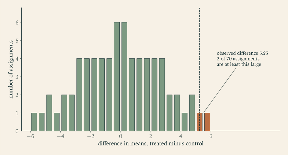
For comparison, the pooled two-sample \(t\) -test on the same data gives \(t\approx2.78\) on \(6\) degrees of freedom and a two-sided p-value of \(0.032\) . The \(t\) -test rests on a normal model; the randomization test does not. That the two are of similar size is typical, and it is one justification for using the \(t\) -test in randomized experiments: it approximates the randomization test, which is the one the design actually justifies. Neyman’s analysis of the same data gives \(\widehat V=7.583/4+6.667/4\approx3.56\) , a standard error of \(1.89\) , and the approximate \(95\%\) interval \(5.25\pm1.96(1.89)=(1.55,\ 8.95)\) for the average effect.
Fisher’s and Neyman’s analyses address different hypotheses. The sharp null says that no unit is affected. Neyman’s null says the average effect is zero, which allows positive effects on some units to cancel negative effects on others. A rejection of the sharp null shows that the treatment does something to some unit; it does not by itself show that the average effect is nonzero, although with a difference-in-means statistic the two usually go together.
12.5 Blocking and pairing
Complete randomization protects against bias. It does not protect against a bad draw, and Example 12.2 showed how large the variance can be when units are heterogeneous. If the experimenter knows in advance which units are alike, that knowledge can be built into the design.
Definition 12.8 (randomized block design). The units are partitioned into blocks \(b=1,\dots,B\) of sizes \(n_b\) , chosen so that units within a block are similar with respect to characteristics expected to affect the outcome. Complete randomization is carried out separately and independently within each block. With \(\hat\tau_b\) the difference in means within block \(b\) , the blocked estimator is
Proposition 12.9 (blocked estimator). In a randomized block design, \(E\,\hat\tau_{\text{blk}}=\tau\) and \(\operatorname{Var}\hat\tau_{\text{blk}}=\sum_b(n_b/n)^2\operatorname{Var}\hat\tau_b\) , where each \(\operatorname{Var}\hat\tau_b\) is given by Theorem 12.5 applied within block \(b\) .
Proof. By Theorem 12.4 applied within each block, \(E\,\hat\tau_b=\tau_b\) , the average effect in block \(b\) , and \(\sum_b(n_b/n)\tau_b=\tau\) because the overall average is the size-weighted average of the block averages. The randomizations in different blocks are independent, so the variances add with the squared weights.
The variance of the blocked estimator involves only the variability of potential outcomes within blocks. Differences between blocks, which under complete randomization would feed into \(S_1^2\) and \(S_0^2\) , contribute nothing, because every block contributes treated and control units in fixed numbers. The guiding principle is: block on what you can, randomize what you cannot. Blocking handles the known sources of variation by design, and randomization within blocks handles the unknown ones.
The extreme case is the matched-pairs design: blocks of two similar units, one of which, chosen by a fair coin, is treated. With \(m\) pairs and within-pair differences \(D_k\) (treated minus control), the estimator is \(\bar D\) , and its variance is estimated by \(s_D^2/m\) , the sample variance of the differences divided by the number of pairs. That estimator is again conservative in the design-based sense. Under the sharp null hypothesis each \(D_k\) is equally likely to have either sign, which gives a randomization test with \(2^m\) equally likely sign patterns.
Example 12.4: Six pairs of plots
Twelve plots are grouped into six pairs of adjacent plots, and within each pair a coin decides which plot receives the fertiliser.
| Pair | 1 | 2 | 3 | 4 | 5 | 6 |
|---|---|---|---|---|---|---|
| Control | \(20\) | \(31\) | \(25\) | \(40\) | \(28\) | \(35\) |
| Treated | \(24\) | \(33\) | \(30\) | \(41\) | \(33\) | \(38\) |
| Difference | \(4\) | \(2\) | \(5\) | \(1\) | \(5\) | \(3\) |
The yields vary greatly from pair to pair, from the twenties to about forty, reflecting differences in soil. The differences vary little. Their mean is \(\bar d=20/6\approx3.33\) and their standard deviation is \(s_D\approx1.633\) , so the standard error is \(1.633/\sqrt6\approx0.667\) and
The \(95\%\) interval for the effect is \(3.33\pm2.571(0.667)=(1.62,\ 5.05)\) . For the randomization test, all six differences are positive, and of the \(2^6=64\) equally likely sign patterns only the observed one gives a mean as large as \(3.33\) : the one-sided p-value is \(1/64\approx0.016\) .
Now analyse the same twelve numbers as if they had come from a completely randomized design, ignoring the pairing. The treated mean is \(33.17\) and the control mean \(29.83\) , the same difference of \(3.33\) ; but the group variances are \(35.8\) and \(51.0\) , the standard error of the difference is \(3.80\) , and \(t\approx0.88\) with a p-value of \(0.40\) . The effect is invisible. The soil differences between pairs, which the paired analysis removes by subtraction, swamp it. The correlation between the two plots of a pair is about \(0.98\) , and it is this correlation that pairing exploits.
The example also carries a warning in the other direction: the analysis must follow the design. A paired experiment analysed as unpaired wastes its precision, as here. An unpaired experiment analysed as if paired, with pairs formed after the fact, has no justification from the randomization at all.
12.6 Planning, and what randomization does not provide
How many units. For a balanced completely randomized experiment with \(n_1=n_0=m\) and outcome standard deviation about \(\sigma\) in each arm, \(\operatorname{Var}\hat\tau\approx2\sigma^2/m\) . Requiring a two-sided level-\(\alpha\) test to have power \(1-\kappa\) against an effect \(\delta\) gives, by the argument of Example 8.1,
For \(\sigma=10\) , \(\delta=5\) , \(\alpha=0.05\) , and power \(0.80\) , this is \(2(1.960+0.842)^2(100)/25\approx62.8\) , so \(63\) units per arm. In a matched-pairs design the relevant variance is that of a within-pair difference, \(2\sigma^2(1-\rho)\) , where \(\rho\) is the within-pair correlation; with \(\rho=0.8\) the requirement falls to about \(12.6\) , that is, \(13\) pairs. A fivefold saving comes from design alone.
How to divide them. If the two arms have different outcome variances, Exercise 7.13 shows that the variance \(S_1^2/n_1+S_0^2/n_0\) is minimised by allocating units in proportion to the standard deviations. Equal allocation is optimal when the variances are equal and is nearly optimal over a wide range.
More than one factor. When two treatments \(A\) and \(B\) are of interest, a factorial experiment assigns each unit at random to one of the four combinations. The same units then serve to estimate the effect of \(A\) , the effect of \(B\) , and their interaction, the extent to which the effect of one depends on the level of the other. Running two separate one-factor experiments would use more units and could not detect the interaction at all (Exercise 18).
What randomization does not do. It justifies inference about the units in the experiment; whether the average effect carries over to other units, times, or conditions is a separate question that the design cannot answer. It guarantees comparability at the moment of assignment; if units drop out, or do not take the treatment they were assigned, the groups actually compared may no longer be the randomized ones. The safe analysis compares the groups as randomized, whatever treatment was actually received. And it balances groups on average; it does not ensure balance in the one experiment performed, which is why blocking on important known variables is worth the trouble.
An experiment produces an estimate of an effect. Often the purpose is then to predict what will happen when the treatment is used, and predictions can be checked against outcomes in a way that estimates of parameters cannot. The final chapter is about that check.
Exercises
-
Define potential outcomes, the unit effect, and the average treatment effect. Explain why no unit effect can be observed, and what assumption about interference between units is built into the notation.
Hint
A unit receives one treatment, so one of \(Y_i(1)\) , \(Y_i(0)\) is observed and the other is counterfactual; their difference needs both. Writing only two potential outcomes per unit assumes that a unit’s outcome does not depend on the treatments given to other units.
-
Four units have potential outcomes \(Y(0)=(5,7,6,10)\) and \(Y(1)=(8,8,9,15)\) . Compute the average treatment effect, list the difference in means for each of the six assignments with two treated units, and verify Theorem 12.4.
Answer
Unit effects \(3,1,3,5\) ; \(\tau=3\) . Differences in means for treated pairs \(\{1,2\},\{1,3\},\{1,4\},\{2,3\},\{2,4\},\{3,4\}\) : \(0,\ 0,\ 5,\ 1,\ 6,\ 6\) . Their average is \(18/6=3=\tau\) .
-
Prove Lemma 12.3, and verify that \(\operatorname{Var}\bigl(\sum_iZ_i\bigr)=0\) , as it must be since the number of treated units is fixed.
Solution
Mean. The assignment is uniform over subsets of size \(n_1\) . By symmetry each unit belongs to the same number of such subsets, so \(P(Z_i=1)\) is the same for all \(i\) ; and \(\sum_iZ_i=n_1\) always, so \(\sum_iP(Z_i=1)=n_1\) and \(E\,Z_i=P(Z_i=1)=n_1/n\) .
Variance. \(Z_i\) is an indicator, so \(\operatorname{Var}Z_i=\frac{n_1}{n}\bigl(1-\frac{n_1}{n}\bigr)=\frac{n_1n_0}{n^2}\) .
Covariance. For \(i\ne j\) , given that unit \(i\) is treated, the other \(n_1-1\) treated units form a uniformly random subset of the remaining \(n-1\) units, so \(P(Z_j=1\mid Z_i=1)=\frac{n_1-1}{n-1}\) . Hence \(E[Z_iZ_j]=\frac{n_1(n_1-1)}{n(n-1)}\) and
\[ \operatorname{Cov}(Z_i,Z_j)=\frac{n_1(n_1-1)}{n(n-1)}-\frac{n_1^2}{n^2}=\frac{n_1\bigl[n(n_1-1)-n_1(n-1)\bigr]}{n^2(n-1)}=\frac{n_1(n_1-n)}{n^2(n-1)}=-\frac{n_1n_0}{n^2(n-1)}. \]The covariance is negative: treating one unit uses up a treatment slot and makes it less likely that any other given unit is treated.
Check. There are \(n\) variance terms and \(n(n-1)\) covariance terms:
\[ \operatorname{Var}\Bigl(\sum_iZ_i\Bigr)=n\cdot\frac{n_1n_0}{n^2}-n(n-1)\cdot\frac{n_1n_0}{n^2(n-1)}=\frac{n_1n_0}{n}-\frac{n_1n_0}{n}=0 , \]as required for a sum that is the constant \(n_1\) . This check in fact determines the covariance: it is the unique common value that makes the variance of the total vanish, the argument used in Exercise 2.18.
-
Use Lemma 12.3 to show that the mean of the \(n_1\) treated units’ values of a fixed variable \(c_1,\dots,c_n\) has variance \(\frac{S_c^2}{n_1}\bigl(1-\frac{n_1}{n}\bigr)\) , where \(S_c^2\) has divisor \(n-1\) , and relate this to Exercise 2.18.
Solution
The mean of the treated units’ values is \(\bar c_T=\frac{1}{n_1}\sum_iZ_ic_i\) . By Lemma 12.3,
\[ \operatorname{Var}\Bigl(\sum_iZ_ic_i\Bigr)=\frac{n_1n_0}{n^2}\sum_ic_i^2-\frac{n_1n_0}{n^2(n-1)}\sum_{i\ne j}c_ic_j . \]Using \(\sum_{i\ne j}c_ic_j=(\sum_ic_i)^2-\sum_ic_i^2\) ,
\[ \sum_ic_i^2-\frac{1}{n-1}\Bigl[\Bigl(\sum_ic_i\Bigr)^2-\sum_ic_i^2\Bigr]=\frac{n}{n-1}\Bigl[\sum_ic_i^2-\frac1n\Bigl(\sum_ic_i\Bigr)^2\Bigr]=n\,S_c^2 , \]since \(\sum_ic_i^2-\frac1n(\sum_ic_i)^2=\sum_i(c_i-\bar c)^2=(n-1)S_c^2\) . Therefore \(\operatorname{Var}(\sum_iZ_ic_i)=\frac{n_1n_0}{n}S_c^2\) , and dividing by \(n_1^2\) ,
\[ \operatorname{Var}\bar c_T=\frac{n_0}{n\,n_1}S_c^2=\frac{S_c^2}{n_1}\Bigl(1-\frac{n_1}{n}\Bigr). \]The factor \(1-n_1/n\) is the finite-population correction: sampling without replacement from a finite set is more precise than independent sampling, and when the whole population is taken, \(n_1=n\) , the mean is known exactly and the variance is zero.
Exercise 2.18 gave \(\operatorname{Var}\bar X=\frac{\sigma^2}{n_1}\cdot\frac{N-n_1}{N-1}\) with \(\sigma^2\) defined with divisor \(N\) . With \(N=n\) and \(\sigma^2=\frac{n-1}{n}S_c^2\) , that is \(\frac{(n-1)S_c^2}{n\,n_1}\cdot\frac{n-n_1}{n-1}=\frac{S_c^2}{n_1}\cdot\frac{n-n_1}{n}\) , the same formula.
-
For the table of Exercise 2, compute \(S_1^2\) , \(S_0^2\) , and \(S_\tau^2\) , evaluate Neyman’s formula, and check it against the variance of the six estimates.
Solution
Variances over the four units. \(Y(1)=(8,8,9,15)\) has mean \(10\) and deviations \(-2,-2,-1,5\) , so \(S_1^2=(4+4+1+25)/3=34/3\approx11.33\) . \(Y(0)=(5,7,6,10)\) has mean \(7\) and deviations \(-2,0,-1,3\) , so \(S_0^2=(4+0+1+9)/3=14/3\approx4.67\) . The effects \((3,1,3,5)\) have mean \(3\) and deviations \(0,-2,0,2\) , so \(S_\tau^2=8/3\approx2.67\) .
Neyman’s formula with \(n_1=n_0=2\) , \(n=4\) .
\[ \operatorname{Var}\hat\tau=\frac{34/3}{2}+\frac{14/3}{2}-\frac{8/3}{4}=\frac{17}{3}+\frac{7}{3}-\frac{2}{3}=\frac{22}{3}\approx7.33 . \]Direct computation. The six equally likely estimates from Exercise 12.2 are \(0,0,5,1,6,6\) , with mean \(3\) and deviations \(-3,-3,2,-2,3,3\) . The squared deviations sum to \(9+9+4+4+9+9=44\) , and \(44/6=22/3\approx7.33\) .
The two agree exactly. The term \(-S_\tau^2/n=-2/3\) is the part that cannot be estimated from one experiment: without it the formula would give \(8\) , which is the expectation of the conservative estimator \(s_1^2/2+s_0^2/2\) . In this table the effects vary from \(1\) to \(5\) , so the treatment changes the spread of outcomes as well as their level, and the conservative estimator overstates the variance by about \(9\%\) .
-
Suppose the treatment adds the same constant to every unit, \(Y_i(1)=Y_i(0)+\tau\) . Show that \(S_\tau^2=0\) and \(S_1^2=S_0^2\) , simplify Neyman’s formula, and explain why the conservative variance estimator is unbiased in this case.
Hint
Adding a constant to every value leaves deviations from the mean unchanged, so \(S_1^2=S_0^2=S^2\) ; the effects are all equal, so \(S_\tau^2=0\) . The formula becomes \(S^2(1/n_1+1/n_0)\) , and \(E\,\widehat V=\operatorname{Var}\hat\tau+0\) .
-
Physicians choose which of their patients receive a new therapy, and the treated patients have better outcomes on average. Write the observed difference in group means in terms of potential outcomes, show that its expectation is the average effect plus a term that vanishes under complete randomization, and interpret that term.
Solution
Let \(T\) be the set of treated patients and \(C\) the set of controls. The observed difference in means is
\[ \frac{1}{n_1}\sum_{i\in T}Y_i(1)-\frac{1}{n_0}\sum_{i\in C}Y_i(0). \]Add and subtract the mean of the untreated potential outcomes of the treated patients, \(\frac{1}{n_1}\sum_{i\in T}Y_i(0)\) :
\[ \underbrace{\frac{1}{n_1}\sum_{i\in T}\bigl(Y_i(1)-Y_i(0)\bigr)}_{\text{average effect among the treated}}\ +\ \underbrace{\frac{1}{n_1}\sum_{i\in T}Y_i(0)-\frac{1}{n_0}\sum_{i\in C}Y_i(0)}_{\text{selection term}} . \]The selection term compares the two groups on the outcome they would have had without the therapy. It measures how different the groups were to begin with.
Under complete randomization \(T\) is a uniformly random subset. The expectation of the first term is \(\tau\) , since the treated are a random sample of all patients, and the expectation of the selection term is \(\bar Y(0)-\bar Y(0)=0\) , since treated and controls are both random samples with respect to \(Y(0)\) . So \(E\,\hat\tau=\tau\) , which is Theorem 12.4 again.
When physicians choose, \(T\) may depend on the potential outcomes. If they give the therapy to patients with better prognosis, the treated have higher \(Y(0)\) on average, the selection term is positive, and the therapy looks better than it is; if they reserve it for the sickest, the term is negative. The first term also changes meaning, becoming the effect among those selected, which need not equal the effect in the whole group. The observed difference is therefore not an unbiased estimate of anything of interest, and the bias cannot be computed from the data, because the \(Y_i(0)\) of treated patients are never observed.
-
An investigator writes: “Because we randomized, the treatment and control groups are identical in every respect, so any difference in outcomes must be caused by the treatment.” Identify what is correct and what is incorrect in this statement, and say what quantity accounts for chance differences between the groups.
Solution
Correct. Randomization ensures that the assignment is unrelated to every characteristic of the units, so there is no systematic difference between the groups: averaged over all possible assignments, the groups are balanced on every variable, observed or not. Consequently the difference in means is an unbiased estimate of the average effect, and treatment is the only systematic cause of a difference in outcomes.
Incorrect. The groups in the experiment actually performed are not identical. One particular assignment was drawn, and by chance it put somewhat healthier, older, or more responsive units in one group. In Example 12.1 the six possible assignments gave estimates from \(-3.5\) to \(9.5\) around a true effect of \(3\) , entirely because of chance imbalance in the units’ potential outcomes. So “any difference in outcomes must be caused by the treatment” is false: part of any observed difference is the luck of the draw.
What accounts for it. The standard error. Chance imbalance is exactly the sampling variability of \(\hat\tau\) under the randomization distribution, quantified by Theorem 12.5 and estimated by \(\widehat V\) . A confidence interval or a randomization test weighs the observed difference against the range of differences that imbalance alone would produce. The correct statement is: because we randomized, a difference larger than chance imbalance can explain is attributable to the treatment. Checking balance on measured covariates is still sensible, since a visible imbalance on an important variable is a reason to adjust for it or, better, to have blocked on it.
-
Six units are completely randomized, three to treatment. The treated outcomes are \(12\) , \(15\) , \(14\) and the control outcomes are \(9\) , \(11\) , \(10\) . Compute the one-sided and two-sided randomization p-values for the difference in means without listing all assignments.
Solution
The six outcomes are \(9,10,11,12,14,15\) , and under the sharp null they are fixed. The observed treated group \(\{12,15,14\}\) consists of the three largest values. The treated mean is \(41/3\approx13.67\) and the control mean is \(10\) , so the observed difference is \(3.67\) .
For any assignment the two group sums add to the fixed total \(71\) , so the difference in means is an increasing function of the treated sum. The treated sum is largest, \(41\) , exactly when the treated group is the three largest values, and since the values are distinct no other choice of three attains it. So among the \(\binom63=20\) equally likely assignments exactly one has a difference at least as large as the observed one:
\[ p_{\text{one-sided}}=\frac{1}{20}=0.05 . \]For the two-sided p-value, count assignments with absolute difference at least \(3.67\) . Exchanging the labels of the two groups reverses the sign of the difference, so the mirror assignment, treating the three smallest values, gives \(-3.67\) , and it is the only one that negative. Hence
\[ p_{\text{two-sided}}=\frac{2}{20}=0.10 . \]With six units the most extreme possible result has a one-sided p-value of exactly \(0.05\) and a two-sided p-value of \(0.10\) . An experiment this small cannot produce two-sided significance at the \(5\%\) level however large the effect, which should be known before it is run.
-
In a balanced completely randomized experiment, what is the smallest total number of units for which a one-sided randomization p-value of at most \(0.05\) is attainable, and the smallest for which \(0.01\) is attainable?
Answer
The smallest attainable one-sided p-value is \(1/\binom{n}{n/2}\) . \(\binom63=20\) gives \(0.05\) , so \(n=6\) . \(\binom84=70\) gives \(0.0143\) , which is too large; \(\binom{10}{5}=252\) gives \(0.004\) , so \(n=10\) .
-
Give an example of a table of potential outcomes for four units in which the average treatment effect is zero but the sharp null hypothesis is false, and explain what a randomization test based on the difference in means is and is not sensitive to in such a case.
Hint
Take unit effects \(+2,+2,-2,-2\) , for instance \(Y(0)=(10,10,10,10)\) and \(Y(1)=(12,12,8,8)\) . The average effect is zero and the sharp null is false. The difference in means has expectation zero, so a test based on it has little power here; a statistic sensitive to spread, such as a difference in variances, would detect the effect.
-
An experiment has two blocks. In block 1, of size four, the treated outcomes are \(20\) , \(22\) and the control outcomes \(17\) , \(19\) . In block 2, of size six, the treated outcomes are \(30\) , \(34\) , \(32\) and the control outcomes \(28\) , \(27\) , \(29\) . Compute the blocked estimate and its conservative standard error, and compare with the standard error obtained by ignoring the blocks.
Solution
Within blocks. Block 1: treated mean \(21\) , control mean \(18\) , \(\hat\tau_1=3\) . Block 2: treated mean \(32\) , control mean \(28\) , \(\hat\tau_2=4\) .
Blocked estimate. With weights \(n_b/n=4/10\) and \(6/10\) ,
\[ \hat\tau_{\text{blk}}=0.4(3)+0.6(4)=3.6 . \]Conservative variance. In block 1 the sample variances are \(2\) (treated: \(20,22\) ) and \(2\) (control: \(17,19\) ), so \(\widehat V_1=2/2+2/2=2\) . In block 2 they are \(4\) (treated: \(30,34,32\) ) and \(1\) (control: \(28,27,29\) ), so \(\widehat V_2=4/3+1/3\approx1.667\) . By Proposition 12.9,
\[ \widehat V_{\text{blk}}=0.4^2(2)+0.6^2(1.667)=0.32+0.60=0.92,\qquad\text{standard error}\approx0.96 . \]Ignoring blocks. The treated outcomes \(20,22,30,34,32\) have mean \(27.6\) and variance \(38.8\) ; the controls \(17,19,28,27,29\) have mean \(24\) and variance \(31\) . The difference is again \(3.6\) , because the proportion treated is the same in both blocks, and
\[ \widehat V=\frac{38.8}{5}+\frac{31}{5}=13.96,\qquad\text{standard error}\approx3.74 . \]The same estimate comes with a standard error almost four times as large. Outcomes in block 2 are about ten units higher than in block 1 whatever the treatment, and the unblocked analysis counts that difference as noise. The blocked analysis is the correct one for this design, since the randomization was carried out within blocks; the unblocked variance describes a design that was not used.
-
In a matched-pairs design let the two units of a pair have outcome variances \(\sigma_1^2\) and \(\sigma_0^2\) and correlation \(\rho\) . Find the variance of the mean of \(m\) within-pair differences, and state when pairing is better than two independent groups of size \(m\) .
Hint
\(\operatorname{Var}(D_k)=\sigma_1^2+\sigma_0^2-2\rho\sigma_1\sigma_0\) , so \(\operatorname{Var}\bar D=(\sigma_1^2+\sigma_0^2-2\rho\sigma_1\sigma_0)/m\) , against \((\sigma_1^2+\sigma_0^2)/m\) for independent groups. Pairing wins when \(\rho>0\) ; it also halves the degrees of freedom for estimating the variance, which matters when \(m\) is small and \(\rho\) is near zero.
-
Find the number of units per arm needed in a balanced completely randomized experiment to detect an effect \(\delta=5\) with \(\sigma=10\) at two-sided level \(0.05\) with power \(0.90\) .
Answer
\(m\ge2(1.960+1.282)^2(100)/25\approx84.1\) , so \(85\) units per arm.
-
The outcome standard deviation is twice as large under treatment as under control. For a fixed total number of units, find the allocation that minimises the variance of the difference in means, and the percentage reduction in variance relative to equal allocation.
Answer
By Exercise 7.13, \(n_1/n_0=\sigma_1/\sigma_0=2\) : two thirds of the units to treatment. The variance is then \((\sigma_1+\sigma_0)^2/n=9\sigma_0^2/n\) , against \(2(\sigma_1^2+\sigma_0^2)/n=10\sigma_0^2/n\) for equal allocation, a reduction of \(10\%\) .
-
Show that in the regression of \(Y\) on an intercept and a binary indicator \(Z\) , the least-squares coefficient of \(Z\) equals the difference between the mean of \(Y\) in the group with \(Z=1\) and the mean in the group with \(Z=0\) .
Solution
Let \(n_1\) units have \(Z_i=1\) and \(n_0=n-n_1\) have \(Z_i=0\) , with group means \(\bar Y_1\) and \(\bar Y_0\) . By the formulas of Section 10.2 the least-squares slope is \(S_{zy}/S_{zz}\) .
Since \(\bar Z=n_1/n\) and \(Z_i^2=Z_i\) ,
\[ S_{zz}=\sum_iZ_i^2-n\bar Z^2=n_1-\frac{n_1^2}{n}=\frac{n_1n_0}{n}. \]Since \(\sum_iZ_iY_i=n_1\bar Y_1\) and \(\sum_iY_i=n_1\bar Y_1+n_0\bar Y_0\) ,
\[ S_{zy}=\sum_iZ_iY_i-\bar Z\sum_iY_i=n_1\bar Y_1-\frac{n_1}{n}\bigl(n_1\bar Y_1+n_0\bar Y_0\bigr)=\frac{n_1n_0}{n}\bigl(\bar Y_1-\bar Y_0\bigr). \]Dividing, the slope is \(\bar Y_1-\bar Y_0\) . The intercept is \(\bar Y-\hat\beta_1\bar Z=\bar Y_0\) , so the fitted values are \(\bar Y_0\) for controls and \(\bar Y_1\) for treated units: the regression reproduces the two group means.
So the difference-in-means estimator is a regression coefficient, and the pooled two-sample \(t\) -test is the \(t\) -test for that coefficient (Exercise 10.13). The interpretation differs with the design. In an observational study the coefficient is subject to the omitted-variable bias of Theorem 10.8. In a completely randomized experiment the same number is unbiased for the average treatment effect by Theorem 12.4, with no linear-model assumption, because the randomization makes \(Z\) unrelated on average to everything else.
-
Eight patients, of whom four are known to be in better health, are assigned by complete randomization, four to treatment. Find the distribution of the number of healthier patients in the treated group, the probability that all four are treated, and the probability that at least three are.
Solution
Label the four healthier patients as “special”. Complete randomization draws \(4\) of the \(8\) patients for treatment, uniformly at random, so the number \(K\) of healthier patients in the treated group is hypergeometric, as in Example 1.5:
\[ P(K=k)=\frac{\binom4k\binom4{4-k}}{\binom84},\qquad k=0,1,2,3,4 . \]The numerators are \(1,16,36,16,1\) and the denominator is \(70\) . The mean is \(4\times\frac48=2\) : on average the healthier patients are split evenly, which is the balance that randomization provides in expectation.
The probability that all four healthier patients are treated is \(1/70\approx0.014\) . The probability that at least three are is \((16+1)/70=17/70\approx0.243\) ; by symmetry the probability that at most one is treated is also \(0.243\) . So a perfectly even split, \(K=2\) , occurs with probability \(36/70\approx0.51\) , and a lopsided split of three to one or worse occurs almost half the time.
This quantifies the caution of Exercise 12.8. Complete randomization with eight units leaves a substantial chance of noticeable imbalance on a variable known to matter. Since the variable is known, the remedy is to block on it: randomize two of the four healthier patients and two of the four others to treatment, which forces \(K=2\) in every assignment and removes health status from the variance of the estimate.
-
A \(2\times2\) factorial experiment gives mean outcomes \(20\) with neither factor, \(26\) with \(A\) only, \(23\) with \(B\) only, and \(35\) with both. Compute the main effect of each factor, averaged over the levels of the other, and the interaction, and explain what two one-factor experiments would have missed.
Answer
Effect of \(A\) : \(\tfrac12\bigl[(26-20)+(35-23)\bigr]=9\) . Effect of \(B\) : \(\tfrac12\bigl[(23-20)+(35-26)\bigr]=6\) . Interaction: \((35-23)-(26-20)=6\) ; the effect of \(A\) is \(12\) when \(B\) is present and \(6\) when it is absent. One-factor experiments run with the other factor absent would report effects \(6\) and \(3\) and predict \(29\) for the combination, missing the extra \(6\) .
-
In a randomized trial some patients assigned to treatment do not take it. Explain why comparing those who took the treatment with those who did not is no longer protected by Theorem 12.4, and what comparison remains protected.
Hint
Whether a patient takes the treatment may depend on prognosis, so the groups “took it” and “did not” are self-selected, and the selection term of Exercise 12.7 need not vanish. The comparison of groups as assigned remains a randomized comparison; it estimates the effect of being assigned to treatment.