Two forecasters issue a probability of rain every morning. The first says “\(30\%\) ” every day, because it rains on about \(30\%\) of days in that city. The second varies: \(5\%\) on some days, \(80\%\) on others. At the end of the year their employer wants to know which of them to keep.
The question is harder than it looks. A single forecast of “\(30\%\) ” is neither right nor wrong when it rains. The first forecaster is never embarrassed and never informative. The second takes risks, and some of them will have gone badly. If the employer rewards whoever was “closest” by some careless measure, the forecasters will learn to shade their reports toward whatever the measure rewards, and the numbers they announce will stop being their real beliefs.
Earlier chapters produced estimates of parameters, which can never be checked against the truth, since the truth is never revealed. A forecast is different: the outcome arrives, and the forecast can be scored. This chapter is about how to do the scoring. It shows that the choice of score determines what a rational forecaster will report, identifies the scores under which honesty is optimal, decomposes a score into the parts that measure calibration and discrimination, and treats the comparison of forecasters as the inference problem it is. It closes by drawing together the methods of the whole book.
13.1 Point forecasts: which summary does the loss reward?
Let \(Y\) be a future observation and suppose a forecaster’s knowledge is described by a predictive distribution \(F\) for \(Y\) . It may be a posterior predictive distribution (Definition 11.9), a fitted model with estimates substituted, or a judgment. A point forecast is a single number \(d\) , and it is evaluated after the fact by a loss \(L(y,d)\) . What should the forecaster report?
Theorem 13.1 (optimal point forecasts). Let \(Y\) have distribution \(F\) with a density and finite variance. The forecast \(d\) minimising the expected loss \(E_F\,L(Y,d)\) is the mean of \(F\) under squared error \((y-d)^2\) ; a median of \(F\) under absolute error \(\lvert y-d\rvert\) ; and the quantile of order \(c_u/(c_u+c_o)\) under the asymmetric linear loss that charges \(c_u\) per unit when \(d<y\) and \(c_o\) per unit when \(d>y\) .
Proof. This is Theorem 11.5 with the predictive distribution \(F\) in place of the posterior distribution and \(Y\) in place of \(\theta\) ; the proof used nothing about the origin of the distribution.
The restriction to distributions with a density is for the proof only. For any distribution with a finite mean, the forecast minimising the asymmetric linear loss is a point \(d\) with \(P(Y<d)\le c_u/(c_u+c_o)\le P(Y\le d)\) , which is how a quantile is defined when the distribution function has jumps; the argument compares the expected loss at \(d\) with that at neighbouring points. For a discrete outcome and the loss that charges \(1\) unless the forecast equals the outcome exactly, the expected loss of forecasting \(d\) is \(1-P(Y=d)\) , so the best forecast is a most probable value, a mode.
The theorem has a consequence for evaluation that is routinely ignored. A request for “a forecast” is ambiguous until the loss is named, because different losses call for different features of \(F\) . If forecasts of a skewed quantity are requested as means and then judged by absolute error, a forecaster who understands the scoring will report medians, and one who honestly reports means will be penalised for it.
Example 13.1: One distribution, two honest forecasts
Daily demand \(Y\) for a spare part is exponentially distributed with mean \(10\) , and two forecasters both know this exactly. The first reports the mean, \(10\) . The second reports the median, \(10\log2\approx6.93\) . Their expected losses are
| Forecast | Mean squared error | Mean absolute error |
|---|---|---|
| mean, \(10\) | \(100.0\) | \(7.36\) |
| median, \(6.93\) | \(109.4\) | \(6.93\) |
Each forecaster wins under the loss for which their summary is optimal and loses under the other. The mean squared error of the median forecast is \(100+(10-6.93)^2\approx109.4\) by Theorem 4.2; the mean absolute error of the mean forecast is \(20/e\approx7.36\) . Neither forecaster knows more than the other. A league table based on absolute error would rank the second above the first, and the ranking would measure only which of them guessed the scoring rule.
If running out of the part costs nine times as much per unit as holding excess stock, the right report is the \(0.9\) quantile, \(10\log10\approx23.0\) , more than twice the mean. Estimation and forecasting share this feature with every decision in Chapter 11: the answer depends on what a mistake costs.
13.2 Probability forecasts and proper scoring rules
Now let the outcome be binary, \(Y\in\{0,1\}\) , and let the forecast be a probability \(q\in[0,1]\) for the event \(Y=1\) .
Definition 13.2 (scoring rule, propriety). A scoring rule assigns a penalty \(S(q,y)\) to the forecast \(q\) when the outcome is \(y\) ; smaller is better. If the event has probability \(p\) , the expected score of reporting \(q\) is
The rule is proper if \(\bar S(p;p)\le\bar S(q;p)\) for all \(p\) and \(q\) , and strictly proper if equality holds only when \(q=p\) .
Under a strictly proper rule a forecaster who believes the probability is \(p\) minimises the expected penalty by reporting exactly \(p\) , and by nothing else. Honesty is the unique best policy. Under an improper rule some other report does better, and a forecaster who understands the rule will give it. Three rules illustrate the definition:
Theorem 13.3 (the Brier score is strictly proper). For the quadratic rule, \(\bar S(q;p)=(q-p)^2+p(1-p)\) .
Proof. \(\bar S(q;p)=p(1-q)^2+(1-p)q^2=p-2pq+q^2\) . Adding and subtracting \(p^2\) gives \((q-p)^2+p-p^2\) .
The expected Brier score splits into a part the forecaster controls, the squared distance between the report and the truth, and a part nobody controls, the intrinsic uncertainty \(p(1-p)\) of the event. It is minimised uniquely at \(q=p\) .
Theorem 13.4 (the logarithmic score is strictly proper). For the logarithmic rule, with the convention \(0\log0=0\) , and for \(0<p<1\) and \(0<q<1\) ,
with equality only when \(q=p\) . In the remaining cases the honest report is again the unique minimiser: if \(0<p<1\) and \(q\) is \(0\) or \(1\) the expected penalty is infinite, and if \(p\) is \(0\) or \(1\) the expected penalty is \(-\log(1-q)\) or \(-\log q\) , which is zero only at \(q=p\) .
Proof. For \(p\) and \(q\) strictly between \(0\) and \(1\) the difference of expected scores is computed directly from the definition. The right side is the Kullback–Leibler divergence from the Bernoulli distribution with probability \(p\) to the one with probability \(q\) , which by Lemma 9.4 is positive unless the two distributions coincide; the moment condition of the lemma holds because both logarithms are bounded. If \(0<p<1\) and \(q=0\) , the event occurs with positive probability and is then penalised by \(-\log0=\infty\) ; the case \(q=1\) is symmetric. If \(p=1\) the event is certain and the penalty is \(-\log q\) , positive for \(q<1\) and zero at \(q=1\) ; the case \(p=0\) is symmetric.
The logarithmic score is the negative log-likelihood of the forecast. Scoring forecasts by it is the predictive counterpart of maximum likelihood, and Lemma 9.4, which explained why maximum likelihood is consistent, is the same fact that makes the score proper. It is severe: a forecast of \(q=0\) for an event that then occurs receives an infinite penalty. A forecaster scored by it must never claim certainty without having it.
Proposition 13.5 (the absolute score is improper). For the absolute rule, \(\bar S(q;p)=p+(1-2p)q\) , which is minimised at \(q=1\) when \(p>1/2\) and at \(q=0\) when \(p<1/2\) .
Proof. \(\bar S(q;p)=p(1-q)+(1-p)q=p+(1-2p)q\) , linear in \(q\) with slope \(1-2p\) . A linear function on \([0,1]\) is minimised at an endpoint: at \(q=1\) if the slope is negative and at \(q=0\) if it is positive.
Under the absolute rule the best report is always \(0\) or \(1\) , whichever side of one half the belief falls on. The rule turns every probability forecast into a categorical call and destroys the information in the probabilities.
Example 13.2: What three rules ask of a forecaster who believes 0.7
Suppose the forecaster’s probability is \(p=0.7\) . The expected penalties for several possible reports are
| Report \(q\) | Brier | Logarithmic | Absolute |
|---|---|---|---|
| \(0.5\) | \(0.250\) | \(0.693\) | \(0.500\) |
| \(0.7\) | \(0.210\) | \(0.611\) | \(0.420\) |
| \(0.9\) | \(0.250\) | \(0.765\) | \(0.340\) |
| \(1.0\) | \(0.300\) | infinite | \(0.300\) |
Under the Brier and logarithmic rules the honest report \(0.7\) has the smallest expected penalty, and exaggerating to \(0.9\) or hedging to \(0.5\) both cost. Under the absolute rule the honest report is beaten by \(0.9\) , and \(0.9\) is beaten by \(1.0\) . Figure 13.1 plots the expected penalty against the report for the three rules. The two proper rules have a minimum at the truth; the improper one slopes all the way to the edge.
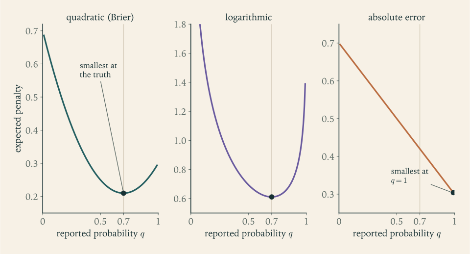
The two proper rules differ in how they punish. The Brier penalty for exaggerating to \(0.9\) equals the penalty for hedging to \(0.5\) ; the logarithmic rule punishes exaggeration more, \(0.765\) against \(0.693\) , because overconfidence risks the large penalty \(-\log(1-q)\) . For outcomes with more than two categories the Brier score becomes \(\sum_j(q_j-\mathbf 1\{y=j\})^2\) and the logarithmic score becomes \(-\log q_y\) , and both remain strictly proper (Exercises 4 and 19).
Common mistake. Judging probability forecasts by “accuracy”, the fraction of occasions on which the event with forecast probability above one half occurred. That is the absolute rule in disguise. It cannot distinguish a forecast of \(0.55\) from one of \(0.99\) , and it rewards rounding every probability to \(0\) or \(1\) .
13.3 Calibration and resolution
A proper score is a single number. To understand why a forecaster scored well or badly it helps to take the number apart. Suppose \(n\) forecasts have been issued, taking \(K\) distinct values \(q_1,\dots,q_K\) . Let \(n_k\) be the number of occasions on which \(q_k\) was issued, \(\bar o_k\) the proportion of those occasions on which the event occurred, and \(\bar o\) the overall proportion of occurrences. The mean Brier score is \(\mathrm{BS}=\frac1n\sum_{t=1}^n(q^{(t)}-y_t)^2\) , where \(q^{(t)}\) is the forecast on occasion \(t\) .
Theorem 13.6 (decomposition of the Brier score).
Proof. Group the occasions by forecast value. Within group \(k\) the outcomes are \(n_k\bar o_k\) ones and \(n_k(1-\bar o_k)\) zeros, so
by the algebra of Theorem 13.3 with \(\bar o_k\) in place of \(p\) . Summing over groups and dividing by \(n\) ,
For the last sum, \(\sum_kn_k\bar o_k=n\bar o\) , and \(\sum_kn_k\bar o_k^2=\sum_kn_k(\bar o_k-\bar o)^2+n\bar o^2\) , so \(\frac1n\sum_kn_k\bar o_k(1-\bar o_k)=\bar o-\bar o^2-\frac1n\sum_kn_k(\bar o_k-\bar o)^2\) .
Each term has a meaning. Reliability measures calibration: whether, among the days on which the forecast was \(q_k\) , the event occurred a fraction \(q_k\) of the time. It is zero for a perfectly calibrated forecaster and it is a penalty. Resolution measures discrimination: how far the outcome frequencies on different kinds of days differ from the overall frequency. It enters with a minus sign: it is a reward. Uncertainty is a property of the events and is the same for every forecaster.
The first forecaster of the opening, who always says the base rate, is perfectly calibrated and has zero resolution, with \(\mathrm{BS}=\bar o(1-\bar o)\) . Calibration alone is cheap. A good forecaster is calibrated and sorts the days into groups with very different outcome frequencies. A plot of \(\bar o_k\) against \(q_k\) , called a reliability diagram, shows calibration as closeness to the diagonal.
Example 13.3: Twenty forecasts taken apart
A forecaster issued \(20\) forecasts using three values, with these results.
| Forecast \(q_k\) | Occasions \(n_k\) | Events | Frequency \(\bar o_k\) |
|---|---|---|---|
| \(0.1\) | \(8\) | \(1\) | \(0.125\) |
| \(0.5\) | \(6\) | \(3\) | \(0.500\) |
| \(0.9\) | \(6\) | \(5\) | \(0.833\) |
Overall \(9\) events occurred in \(20\) occasions, so \(\bar o=0.45\) and the uncertainty is \(0.45\times0.55=0.2475\) . Directly, the squared errors sum to \((7\times0.01+0.81)+6\times0.25+(5\times0.01+0.81)=3.24\) , so \(\mathrm{BS}=0.162\) . The components are
and \(0.0016-0.0871+0.2475=0.162\) , as the theorem requires. The forecaster is well calibrated, with a reliability penalty of almost nothing, and has substantial resolution. A forecaster who always said \(0.45\) would have scored \(0.2475\) . The skill score \(1-\mathrm{BS}/\bigl(\bar o(1-\bar o)\bigr)=1-0.162/0.2475\approx0.35\) expresses the improvement over that reference as a fraction.
13.4 Comparing forecasters is an inference problem
The Brier score \(0.162\) beats the reference \(0.2475\) . Is that skill, or luck over \(20\) occasions? A mean score is a sample mean, and it has a standard error.
Let \(d_t=S(q_t^A,y_t)-S(q_t^B,y_t)\) be the difference in penalties of forecasters \(A\) and \(B\) on occasion \(t\) , with mean \(\bar d\) and sample standard deviation \(s_d\) . If the differences behave like independent draws from a common distribution, the Central Limit Theorem gives the approximate pivot \(\sqrt n(\bar d-\delta)/s_d\) , where \(\delta\) is the expected score difference, and hence the test statistic \(\sqrt n\,\bar d/s_d\) for the hypothesis of equal expected scores and the interval \(\bar d\pm z_{\alpha/2}s_d/\sqrt n\) . This is a paired comparison in the sense of Section 12.5: both forecasters face the same events, and differencing removes the variation in how hard each occasion was to forecast. It is essential to use a proper scoring rule here, or the test would compare the forecasters’ gamesmanship.
Example 13.4: Is the forecaster better than the base rate?
Compare the forecaster of Example 13.3, as \(B\) , with the reference \(A\) that always reports \(0.45\) . The reference’s penalty is \(0.3025\) when the event occurs and \(0.2025\) when it does not. The \(20\) differences take six values: \(0.1925\) on the seven quiet days forecast at \(0.1\) , \(-0.5075\) on the one such day when the event occurred, \(0.0525\) and \(-0.0475\) on the three event days and three non-event days forecast at \(0.5\) , \(0.2925\) on the five event days forecast at \(0.9\) , and \(-0.6075\) on the one such day without the event. Their mean is \(\bar d=0.2475-0.162=0.0855\) and their standard deviation is \(s_d\approx0.2495\) . Then
with a two-sided p-value of about \(0.14\) from the \(t_{19}\) distribution. An improvement of a third in the Brier score, over twenty occasions, is not distinguishable from chance. The two occasions on which a confident forecast failed dominate the variance. By the sample-size formula of Section 8.1, detecting a true difference of this size with power \(0.8\) at the two-sided \(5\%\) level would take about \(\bigl((1.960+0.842)\times0.2495/0.0855\bigr)^2\approx67\) forecasts.
The independence assumption deserves suspicion. Forecast errors on successive days are often correlated, and when forecasts are made several steps ahead, errors for overlapping periods are correlated by construction. Positive correlation makes \(s_d/\sqrt n\) too small, and the standard error must then be computed with an allowance for the autocovariances of the \(d_t\) ; the test with that correction is known as the Diebold–Mariano test.
13.5 In-sample fit is not forecast performance
A model can be evaluated on the data used to fit it or on new data. The first is easier and biased in a known direction.
Theorem 13.7 (optimism of the in-sample error). In the linear model \(y=X\beta+\varepsilon\) with \(p\) parameters, satisfying (A2), let \(\hat y=X\hat\beta\) be the least-squares fit, and let \(y^\ast=X\beta+\varepsilon^\ast\) be an independent new set of responses at the same design points. Then
Proof. The first statement is Theorem 10.4: \(E\,\mathrm{RSS}=(n-p)\sigma^2\) . For the second, \(y^\ast-\hat y=\varepsilon^\ast-H\varepsilon\) , since \(\hat y=X\beta+H\varepsilon\) . The two terms are independent with mean zero, so the expected squared length is \(E\lVert\varepsilon^\ast\rVert^2+E\lVert H\varepsilon\rVert^2=n\sigma^2+\sigma^2\operatorname{tr}(H)=(n+p)\sigma^2\) , using \(E\lVert H\varepsilon\rVert^2=\sigma^2\operatorname{tr}(H^{\top}H)=\sigma^2\operatorname{tr}(H)=p\sigma^2\) .
The gap between the two is \(2p\sigma^2/n\) . Fitting uses the noise in the training responses to reduce the residuals, so the residuals understate the error, and each additional parameter both lowers the in-sample error and raises the out-of-sample error by \(\sigma^2/n\) . Choosing among models by in-sample fit therefore always favours the largest model. Honest evaluation requires data not used in fitting: a held-out set, or cross-validation, in which each observation in turn is predicted from a fit to the others.
Example 13.5: Polynomials for the fertiliser data
For the eight plots of Example 10.1, fit polynomials of degree \(1\) to \(5\) and record the in-sample mean squared error \(\mathrm{RSS}/n\) and the leave-one-out cross-validated mean squared error.
| Degree | Parameters | In-sample MSE | Leave-one-out MSE |
|---|---|---|---|
| 1 | 2 | \(0.231\) | \(0.406\) |
| 2 | 3 | \(0.228\) | \(0.517\) |
| 3 | 4 | \(0.228\) | \(1.48\) |
| 4 | 5 | \(0.228\) | \(15.5\) |
| 5 | 6 | \(0.017\) | \(2.13\) |
The in-sample error never increases with the degree and collapses at degree \(5\) , where six parameters are fitted to eight points. The cross-validated error is smallest for the straight line and larger for every higher degree, by a factor of nearly forty at degree \(4\) ; the wiggles of the higher-degree fits follow the noise and predict the omitted point badly. For the line, Theorem 13.7 predicts the pattern: with \(\hat\sigma^2=0.3076\) , the expected in-sample error is \(0.3076(1-2/8)\approx0.231\) , which is \(\mathrm{RSS}/n\) exactly, and the expected error for new responses is \(0.3076(1+2/8)\approx0.385\) , close to the cross-validated \(0.406\) .
13.6 Forecast distributions for continuous outcomes
For a continuous outcome a full forecast is a predictive density \(f\) , and the logarithmic score \(-\log f(y)\) is again strictly proper, by Lemma 9.4. Two simpler forms of forecast are common, and each has its own check.
Interval forecasts. A \(95\%\) prediction interval should contain the outcome \(95\%\) of the time, and among intervals with correct coverage, narrower is better. Coverage can be verified against outcomes, and it frequently fails because parameter uncertainty was ignored. For a normal sample of size \(n\) , the interval \(\bar x\pm1.96\,s\) , which substitutes estimates for \(\mu\) and \(\sigma\) , has actual coverage \(P\bigl(\lvert t_{n-1}\rvert\le1.96/\sqrt{1+1/n}\bigr)\) by Proposition 7.6. For \(n=9\) that is \(P(\lvert t_8\rvert\le1.859)\approx0.90\) : a nominal \(95\%\) interval that misses twice as often as claimed. The interval of Proposition 7.6, and the posterior predictive distribution of Definition 11.9, repair this by carrying the uncertainty about the parameters into the forecast.
Calibration of a predictive distribution. If the predictive distribution functions \(F_t\) are correct, then by Proposition 2.10 the values \(F_t(y_t)\) , called probability integral transforms, are uniformly distributed on \((0,1)\) . A histogram of them should be flat. A U-shaped histogram, with too many values near \(0\) and \(1\) , means the outcomes fall in the tails of the forecasts too often: the forecast distributions are too narrow. A hump in the middle means they are too wide, and a slope means they are biased. This is the continuous analogue of the reliability diagram.
13.7 Choosing the tool
The thirteen chapters have assembled a set of procedures, and using them well consists largely in recognising which question is being asked. The table gathers the main ones.
| Question | Procedure | What it guarantees | What it assumes |
|---|---|---|---|
| Can the quantity be learned at all? | identifiability check (Ch. 1) | necessary for consistency | the model family |
| What single value? | MLE (Ch. 5); UMVUE (Ch. 6); Bayes estimate (Ch. 11) | asymptotic efficiency; least variance among unbiased; least average risk | regularity; complete sufficient statistic; prior and loss |
| What range of values? | confidence set by pivot (Ch. 7) or large-sample pivot (Ch. 9); credible set (Ch. 11) | coverage for every parameter value; posterior probability | exact or approximate sampling distribution; prior |
| Is a specific value tenable? | test, p-value (Ch. 8, 9) | type I error rate | null distribution; hypothesis fixed in advance |
| How does a mean depend on covariates? | linear model (Ch. 10) | unbiased, exact \(t\) and \(F\) inference | linearity, equal variances, normality, checked by residuals |
| What does an intervention do? | randomized experiment (Ch. 12) | unbiased effect estimate, exact test | random assignment, no interference |
| What will happen next? | prediction interval (Ch. 7, 10); predictive distribution (Ch. 11) | coverage for the new observation | model, plus parameter uncertainty carried through |
| How good was the forecast? | proper scoring rule (Ch. 13) | honesty is optimal | score chosen before forecasts are seen |
Three habits run through all of them. State the model and the estimand before computing, and check that the estimand is identifiable. Attach to every number a statement of its uncertainty, and say what kind of statement it is: a frequency over repeated samples, a posterior probability, a randomization distribution. And examine the assumptions with the data in hand, through residuals, sensitivity to the prior, exact calculations at the actual sample size, or scores on held-out outcomes, because every guarantee in this book is conditional on a model, and the model is the part that the mathematics cannot certify.
Exercises
-
Define a scoring rule, its expected score, and propriety. Compute the Brier and logarithmic penalties of the forecast \(q=0.8\) when the event occurs and when it does not.
Answer
Event occurs: Brier \((0.8-1)^2=0.04\) , logarithmic \(-\log0.8\approx0.223\) . Event does not occur: Brier \(0.64\) , logarithmic \(-\log0.2\approx1.609\) .
-
A future count \(Y\) takes the values \(0,1,2,10\) with probabilities \(0.4,0.3,0.2,0.1\) . Find the optimal point forecast under squared error, under absolute error, and under the zero-one loss that charges \(1\) unless the forecast is exactly right.
Answer
Squared error: the mean, \(0.3+0.4+1.0=1.7\) . Absolute error: the median, \(1\) , since \(P(Y<1)=0.4\le0.5\le P(Y\le1)=0.7\) , by the remark after Theorem 13.1. Zero-one loss: the expected loss of forecasting \(d\) is \(1-P(Y=d)\) , smallest at the mode, \(0\) . Three losses, three forecasts, none of them wrong.
-
For the exponential demand of Example 13.1, find the optimal forecast when a unit of shortfall costs \(9\) and a unit of excess costs \(1\) , and explain why a forecaster rewarded for small mean squared error would not report it.
Answer
The quantile of order \(9/(9+1)=0.9\) : \(10\log10\approx23.0\) . Under mean squared error the optimal report is the mean, \(10\) ; reporting \(23.0\) would have mean squared error \(100+13.0^2\approx270\) . A forecaster follows the loss that determines the reward.
-
Let \(Y\) take one of three categories with probabilities \(p=(p_1,p_2,p_3)\) and let a forecast be a probability vector \(q\) . Prove that the expected value of \(\sum_{j=1}^3(q_j-\mathbf 1\{Y=j\})^2\) equals \(\sum_j(q_j-p_j)^2+\sum_jp_j(1-p_j)\) , and conclude that this score is strictly proper.
Solution
Fix a category \(j\) . The indicator \(\mathbf 1\{Y=j\}\) is a Bernoulli variable with success probability \(p_j\) , so by the calculation of Theorem 13.3,
\[ E\bigl(q_j-\mathbf 1\{Y=j\}\bigr)^2=p_j(q_j-1)^2+(1-p_j)q_j^2=(q_j-p_j)^2+p_j(1-p_j). \]The expectation of a sum is the sum of the expectations, whether or not the three indicators are independent (they are not: exactly one of them equals one). Summing over \(j\) ,
\[ E\sum_{j=1}^3\bigl(q_j-\mathbf 1\{Y=j\}\bigr)^2=\sum_{j=1}^3(q_j-p_j)^2+\sum_{j=1}^3p_j(1-p_j). \]The second sum does not involve the forecast. The first is the squared Euclidean distance between \(q\) and \(p\) ; it is nonnegative and equals zero only when \(q_j=p_j\) for every \(j\) . Hence the expected score is minimised by \(q=p\) and by no other probability vector: the multi-category Brier score is strictly proper.
The argument works for any number of categories. The term \(\sum_jp_j(1-p_j)\) is the irreducible part, largest when the categories are equally likely and zero when the outcome is certain. Note that the minimisation did not even need the constraint that \(q\) sum to one: the unconstrained minimiser already satisfies it.
-
Consider the rule \(S(q,y)=(q-y)^4\) for a binary event. Find the report that minimises the expected penalty when the event has probability \(p\) , show that the rule is improper, and evaluate the optimal report for \(p=0.7\) .
Solution
The expected penalty of reporting \(q\) is
\[ \bar S(q;p)=p(1-q)^4+(1-p)q^4 . \]Its second derivative \(12p(1-q)^2+12(1-p)q^2\) is positive, so the function is strictly convex on \([0,1]\) and has a unique minimiser, found by setting the first derivative to zero:
\[ -4p(1-q)^3+4(1-p)q^3=0\quad\Longleftrightarrow\quad\Bigl(\frac{q}{1-q}\Bigr)^3=\frac{p}{1-p}. \]So the optimal report \(q^\ast\) has odds equal to the cube root of the true odds:
\[ \frac{q^\ast}{1-q^\ast}=\Bigl(\frac{p}{1-p}\Bigr)^{1/3}. \]This equals \(p\) only when the odds are \(0\) , \(1\) , or infinite, that is, when \(p\in\{0,\tfrac12,1\}\) . For every other \(p\) the best report differs from the belief, so the rule is improper.
For \(p=0.7\) the true odds are \(7/3\approx2.333\) , the cube root is about \(1.326\) , and \(q^\ast=1.326/2.326\approx0.570\) .
The direction of the distortion is the opposite of the absolute rule’s. The fourth power punishes large errors so heavily that the forecaster hedges toward \(1/2\) to avoid them, reporting \(0.57\) while believing \(0.7\) . The absolute rule pushes reports to the extremes, the fourth-power rule pulls them to the middle, and only the square, among powers of \(\lvert q-y\rvert\) , leaves them where they belong.
-
A forecasting contest scores entrants by the mean absolute error \(\lvert q-y\rvert\) . An entrant believes each of a series of events has probability \(0.6\) . What should the entrant report to minimise the expected penalty, what is the gain over honest reporting, and what does the organiser lose?
Solution
By Proposition 13.5 the expected absolute penalty of reporting \(q\) when the belief is \(p\) is \(p+(1-2p)q\) . With \(p=0.6\) this is \(0.6-0.2q\) , decreasing in \(q\) , so the best report is \(q=1\) , with expected penalty \(0.4\) . The honest report \(q=0.6\) has expected penalty \(0.6-0.12=0.48\) . Declaring certainty lowers the expected penalty by \(0.08\) per event, a reduction of one sixth.
The entrant who wants to win should therefore report \(1\) for every event believed more likely than not, and \(0\) for every event believed less likely than not. An entrant who believes \(0.51\) and one who believes \(0.99\) submit the same number.
The organiser loses the thing the contest was meant to elicit. The submitted “probabilities” are all \(0\) or \(1\) ; they carry only the information of which side of one half each entrant’s belief lies on. Calibration cannot be assessed, because nobody reports intermediate values. And the ranking rewards the willingness to exaggerate as much as it rewards knowledge: an honest, well-calibrated entrant is systematically beaten by one with the same beliefs who rounds them. Replacing the rule with the Brier or logarithmic score removes the incentive at no cost, since under either the report \(0.6\) is uniquely optimal for a belief of \(0.6\) .
-
An event has probability \(0.9\) . Compute the expected logarithmic penalty of the honest forecast and of the overconfident forecast \(0.99\) , and explain the size of the difference.
Answer
Honest: \(-(0.9\log0.9+0.1\log0.1)\approx0.325\) . Overconfident: \(-(0.9\log0.99+0.1\log0.01)\approx0.470\) . The forecast \(0.99\) gains almost nothing on the nine occasions in ten when the event occurs and pays \(-\log0.01\approx4.6\) on the tenth.
-
A forecaster issued \(q=0.2\) on ten occasions, on three of which the event occurred, and \(q=0.7\) on ten occasions, on six of which it occurred. Compute the mean Brier score directly and from its reliability, resolution, and uncertainty components.
Solution
Directly. In the first group the forecast is \(0.2\) : seven non-events each contribute \(0.2^2=0.04\) and three events each contribute \(0.8^2=0.64\) , a total of \(0.28+1.92=2.20\) . In the second group the forecast is \(0.7\) : six events each contribute \(0.09\) and four non-events each contribute \(0.49\) , a total of \(0.54+1.96=2.50\) . Hence
\[ \mathrm{BS}=\frac{2.20+2.50}{20}=0.235 . \]By components. The group frequencies are \(\bar o_1=0.3\) and \(\bar o_2=0.6\) , and overall \(\bar o=9/20=0.45\) .
\[ \text{reliability}=\frac{10(0.2-0.3)^2+10(0.7-0.6)^2}{20}=\frac{0.1+0.1}{20}=0.010, \]\[ \text{resolution}=\frac{10(0.3-0.45)^2+10(0.6-0.45)^2}{20}=\frac{0.225+0.225}{20}=0.0225, \]and the uncertainty is \(0.45\times0.55=0.2475\) . Then \(0.010-0.0225+0.2475=0.235\) , in agreement.
This forecaster is only slightly better than the constant forecast \(0.45\) , whose score is \(0.2475\) . The reliability term shows a consistent miscalibration, each forecast being \(0.1\) too extreme, and the resolution is small because the two groups of days, with frequencies \(0.3\) and \(0.6\) , are not very different. Compare Example 13.3, where the same uncertainty came with a resolution of \(0.087\) .
-
For the forecaster of Exercise 8, suppose each forecast is replaced by the observed frequency in its group. Compute the new mean Brier score, show that such recalibration can never increase the score on the same data, and explain why the improvement is not evidence about future performance.
Solution
Replacing \(0.2\) by \(0.3\) and \(0.7\) by \(0.6\) leaves the grouping of occasions unchanged, so the group frequencies \(\bar o_k\) and the resolution are unchanged, and the reliability becomes \(\frac1n\sum_kn_k(\bar o_k-\bar o_k)^2=0\) . By Theorem 13.6 the new score is
\[ \mathrm{BS}=0-0.0225+0.2475=0.225 , \]down from \(0.235\) .
In general, recalibration to the group frequencies changes the score from reliability minus resolution plus uncertainty to minus resolution plus uncertainty. Since the reliability term is a sum of squares, it is nonnegative, and removing it can never increase the score. If two groups happen to share the same frequency they merge after recalibration, which leaves the resolution sum unchanged as well.
The improvement is an in-sample result. The frequencies \(0.3\) and \(0.6\) were estimated from ten occasions each, with standard errors of about \(0.15\) , and then used to score the very outcomes they were estimated from. This is the optimism of Theorem 13.7 in another setting: a quantity tuned to the data is evaluated on the same data. On new occasions the recalibrated forecasts will show a positive reliability term again, because the true frequencies differ from the estimates. To learn whether recalibration helps, apply the map estimated on these twenty occasions to a fresh set and score that.
-
Show that a forecaster who always reports the overall event frequency \(\bar o\) has reliability zero, resolution zero, and mean Brier score \(\bar o(1-\bar o)\) , and compute the skill score of the forecaster of Example 13.3 relative to this reference.
Answer
There is one group, with \(q_1=\bar o_1=\bar o\) , so both sums of squares vanish and \(\mathrm{BS}=\bar o(1-\bar o)\) . For Example 13.3 the skill score is \(1-0.162/0.2475\approx0.35\) .
-
Suppose a forecaster is perfectly calibrated: among occasions on which the forecast is \(q\) , the event has probability \(q\) . Show that the expected Brier score is the average of \(q(1-q)\) over the forecasts issued, and deduce which of two calibrated forecasters scores better.
Solution
Condition on the forecast. On occasions when the forecast is \(q\) , calibration says the event is a Bernoulli variable with probability \(q\) , so by Theorem 13.3 with \(p=q\) the expected penalty is
\[ E\bigl[(q-Y)^2\mid q\bigr]=(q-q)^2+q(1-q)=q(1-q). \]Averaging over the forecasts issued, the expected Brier score of a calibrated forecaster is the average of \(q(1-q)\) , written \(E[q(1-q)]\) .
The function \(q(1-q)\) is largest at \(q=1/2\) and zero at \(q=0\) and \(q=1\) . So among calibrated forecasters, the one whose forecasts lie closer to \(0\) and \(1\) scores better. This property of the forecasts alone is called sharpness. More precisely, calibration implies that the average forecast equals the overall event frequency \(\bar o\) , and then
\[ E[q(1-q)]=E\,q-E\,q^2=\bar o-\bigl(\operatorname{Var}(q)+\bar o^2\bigr)=\bar o(1-\bar o)-\operatorname{Var}(q). \]The expected score is the uncertainty minus the variance of the forecasts. For a calibrated forecaster the variance of the forecasts is the resolution. Of two calibrated forecasters facing the same events, the one whose forecasts vary more scores better. The base-rate forecaster has variance zero and the worst score a calibrated forecaster can have. The goal of probability forecasting can be summarised as: maximise sharpness subject to calibration.
-
Ten paired score differences between two forecasters are \(0.10\) , \(-0.02\) , \(0.15\) , \(0.05\) , \(0.08\) , \(-0.04\) , \(0.12\) , \(0.03\) , \(0.09\) , \(0.04\) . Compute the mean, the standard deviation, and the \(t\) statistic for equal expected scores, and state the assumption on which the p-value depends.
Answer
Mean \(0.060\) ; standard deviation \(0.060\) ; \(t=\sqrt{10}\times0.060/0.060\approx3.16\) on \(9\) degrees of freedom, two-sided p-value about \(0.012\) . The p-value assumes that the ten differences are independent with a common distribution; serial correlation between occasions would invalidate the standard error.
-
Verify Theorem 13.7 directly for the model with an intercept only, \(p=1\) : show that \(E\bigl[\frac1n\sum(Y_i-\bar Y)^2\bigr]=\sigma^2(1-\frac1n)\) and that the expected squared error of \(\bar Y\) as a forecast of an independent new observation is \(\sigma^2(1+\frac1n)\) .
Solution
Let \(Y_1,\dots,Y_n\) be uncorrelated with mean \(\mu\) and variance \(\sigma^2\) . The intercept-only model has \(p=1\) , fitted value \(\bar Y\) for every observation, and hat matrix with all entries \(1/n\) .
In-sample. By Theorem 2.2, \(E\sum(Y_i-\bar Y)^2=(n-1)\sigma^2\) , so
\[ E\Bigl[\frac1n\sum_{i=1}^n(Y_i-\bar Y)^2\Bigr]=\frac{n-1}{n}\sigma^2=\sigma^2\Bigl(1-\frac1n\Bigr), \]which is the first formula of Theorem 13.7 with \(p=1\) .
Out-of-sample. Let \(Y^\ast\) be a new observation with the same mean and variance, independent of the sample. Then \(Y^\ast-\bar Y\) has mean zero, and by independence
\[ E(Y^\ast-\bar Y)^2=\operatorname{Var}Y^\ast+\operatorname{Var}\bar Y=\sigma^2+\frac{\sigma^2}{n}=\sigma^2\Bigl(1+\frac1n\Bigr), \]the second formula with \(p=1\) . Averaging over \(n\) new observations, one at each design point, gives the same value.
The two differ by \(2\sigma^2/n\) . The reason is visible here in the simplest possible form. \(\bar Y\) is the value that minimises \(\sum(Y_i-c)^2\) over \(c\) , so it is closer to the sample than \(\mu\) is, and the in-sample error is below \(\sigma^2\) . But \(\bar Y\) is not \(\mu\) , and its own error \(\sigma^2/n\) is added when it is used to predict something new. The divisor \(n-1\) of the sample variance and the factor \(1+1/n\) in the prediction interval of Proposition 7.6 are the two halves of this theorem.
-
For a linear model with \(n=20\) observations and \(p=5\) parameters, find the ratio of the expected out-of-sample error to the expected in-sample error given by Theorem 13.7, and say what it implies for a model chosen by in-sample fit.
Answer
\((1+5/20)/(1-5/20)=1.25/0.75\approx1.67\) . New data will show errors about two thirds larger than the residuals suggest, and comparing models of different sizes by their residuals favours the larger model by the full difference \(2p\sigma^2/n\) .
-
A forecaster issues the predictive distribution \(N(0,1)\) on every occasion, but the outcomes are in fact \(N(0,4)\) . Find the distribution function of the probability integral transform, describe the shape of its histogram, and compute the fraction of outcomes falling outside the forecaster’s central \(90\%\) intervals.
Solution
The forecaster’s predictive distribution function is \(\Phi\) , so the probability integral transform is \(U=\Phi(Y)\) . The outcome is \(Y=2Z\) with \(Z\) standard normal. For \(0<u<1\) ,
\[ P(U\le u)=P\bigl(Y\le\Phi^{-1}(u)\bigr)=P\bigl(Z\le\tfrac12\Phi^{-1}(u)\bigr)=\Phi\bigl(\tfrac12\Phi^{-1}(u)\bigr). \]If the forecasts were correct this would equal \(u\) . Instead, for \(u<1/2\) the argument \(\tfrac12\Phi^{-1}(u)\) is closer to zero than \(\Phi^{-1}(u)\) , so \(P(U\le u)>u\) : there is too much probability near \(0\) , and by symmetry too much near \(1\) . Differentiating, the density of \(U\) is \(\tfrac12\phi\bigl(\tfrac12\Phi^{-1}(u)\bigr)/\phi\bigl(\Phi^{-1}(u)\bigr)\) , which equals \(1/2\) at \(u=1/2\) and grows without bound as \(u\to0\) or \(u\to1\) . The histogram is U-shaped.
The forecaster’s central \(90\%\) interval is \(\pm1.645\) . The outcome falls outside it when \(\lvert2Z\rvert>1.645\) , that is, when \(\lvert Z\rvert>0.822\) :
\[ P(\lvert Z\rvert>0.822)=2\Phi(-0.822)\approx0.411 . \]Intervals claimed to miss \(10\%\) of the time miss \(41\%\) of the time. The forecast distributions are too narrow by a factor of two in standard deviation, and the U-shaped histogram of transforms is the signature of that overconfidence; equivalently, \(P(U\le0.05)=\Phi(-0.822)\approx0.205\) where \(0.05\) was promised.
-
For a normal sample of size \(5\) , compute the actual coverage of the plug-in forecast interval \(\bar x\pm1.96\,s\) for a new observation, and give the multiplier of \(s\) that achieves \(95\%\) coverage.
Solution
By Proposition 7.6, \((X_6-\bar X)/(S\sqrt{1+1/5})\sim t_4\) . The plug-in interval contains the new observation when \(\lvert X_6-\bar X\rvert\le1.96\,S\) , that is, when
\[ \lvert t_4\rvert\le\frac{1.96}{\sqrt{1.2}}\approx1.789 . \]The coverage is \(P(\lvert t_4\rvert\le1.789)\approx0.852\) . The nominal \(95\%\) interval misses about \(15\%\) of new observations, three times the stated rate.
Two separate errors are being made. Treating \(\bar x\) as \(\mu\) ignores the factor \(\sqrt{1+1/n}\) , and treating \(s\) as \(\sigma\) ignores the heavier tails of \(t_4\) compared with the normal. For \(95\%\) coverage the half-width must be \(t_{4,0.025}\sqrt{1.2}\,s=2.776\times1.095\,s\approx3.04\,s\) , more than one and a half times the plug-in multiplier \(1.96\) .
Each error shrinks as \(n\) grows, but slowly: for \(n=9\) the plug-in coverage is \(0.90\) and for \(n=30\) it is still only about \(0.936\) . A forecast interval that substitutes estimates for parameters and ignores the substitution is overconfident, and the shortfall in coverage is exactly the kind of miscalibration that the checks of Section 13.6 are designed to reveal.
-
In Example 11.6, compare the posterior predictive probability and the plug-in probability of the outcome \(Y=0\) by their logarithmic penalties if that outcome occurs, and explain, using Theorem 13.4, which forecast has the smaller expected penalty if the posterior describes the uncertainty correctly.
Hint
If \(Y=0\) occurs the penalties are \(-\log0.302\approx1.20\) and \(-\log0.263\approx1.34\) . If the posterior is a correct description, the true distribution of \(Y\) given the data is the posterior predictive distribution, so the event \(Y=0\) has probability \(0.302\) . By Theorem 13.4, applied to that binary event, reporting \(0.302\) has a smaller expected logarithmic penalty than reporting \(0.263\) ; Exercise 13.19 extends the comparison to the whole distribution of \(Y\) .
-
For each situation name the appropriate procedure from the table in Section 13.7 and the assumption most in need of checking: (a) a manufacturer wants a guaranteed-coverage range for the mean breaking strength from twelve specimens; (b) a clinic wants to know whether a reminder letter increases attendance; (c) an analyst has three candidate models for monthly sales and wants to pick one for next year’s forecasts.
Answer
(a) A \(t\) confidence interval for the mean (Chapter 7); check approximate normality and independence of the specimens, since twelve observations give the Central Limit Theorem little to work with. (b) A randomized experiment with a comparison of attendance proportions (Chapter 12); check that assignment really was random and that one patient’s letter cannot affect another’s attendance. (c) Out-of-sample evaluation with a proper score or cross-validation (Chapter 13); check that the evaluation data were not used in fitting or selecting the models, and allow for serial dependence in monthly data.
-
Let \(p\) and \(q\) be probability mass functions on a finite set. Show that the expected logarithmic penalty of forecast \(q\) when \(p\) is true exceeds that of forecast \(p\) by \(\sum_yp(y)\log\bigl(p(y)/q(y)\bigr)\) , and deduce from Lemma 9.4 that the logarithmic score is strictly proper for outcomes with any finite number of categories.
Hint
The expected penalties are \(-\sum_yp(y)\log q(y)\) and \(-\sum_yp(y)\log p(y)\) ; subtract. The difference is the Kullback–Leibler divergence, and Lemma 9.4, applied to mass functions with sums in place of integrals, shows it is positive unless \(q=p\) .