Sample the function \(f(x)=1/(1+25x^2)\) at eleven equally spaced points of \([-1,1]\) and pass the polynomial of degree \(10\) through the samples. The polynomial agrees with \(f\) at every sample, as it must, and between the samples near the ends of the interval it swings away so violently that the largest discrepancy is \(1.92\) , almost twice the maximum of \(f\) itself. Take more samples to fix it: with \(21\) equally spaced points the largest discrepancy is \(59.8\) , and with \(41\) it is about \(10^{5}\) . More data made the approximation worse.
Now keep the number of samples but move them. With eleven points crowded toward the ends of the interval in a particular way, the discrepancy is \(0.109\) ; with \(21\) it is \(0.0153\) ; with \(41\) it is \(2.9\times10^{-4}\) , and it keeps shrinking geometrically. The same function, the same kind of polynomial, the same amount of information: one arrangement diverges and the other converges.
This chapter explains both outcomes with one formula. Interpolation replaces a function known at a few points by a polynomial, and the questions are the ones Chapter 1 taught us to ask of any computation. Is the problem well posed? How large is the truncation error, and what controls it? How sensitive is the result to errors in the data? The answers involve the function and the placement of the points separately, and the second is ours to choose.
4.1 One polynomial, several disguises
Write \(\mathcal P_n\) for the set of polynomials of degree at most \(n\) .
Theorem 4.1 (existence and uniqueness of the interpolating polynomial). Let \(x_0,x_1,\dots,x_n\) be distinct real numbers and \(y_0,\dots,y_n\) arbitrary real numbers. There is exactly one polynomial \(p\in\mathcal P_n\) with \(p(x_j)=y_j\) for \(j=0,\dots,n\) .
Proof. Uniqueness. If \(p\) and \(q\) both qualify, \(p-q\in\mathcal P_n\) vanishes at the \(n+1\) distinct points \(x_j\) . A nonzero polynomial of degree at most \(n\) has at most \(n\) roots, so \(p-q\) is the zero polynomial. Existence. For each \(j\) define
Each \(\ell_j\) has degree \(n\) , equals \(1\) at \(x_j\) , and vanishes at every other node. Therefore \(p(x)=\sum_{j=0}^{n}y_j\,\ell_j(x)\) lies in \(\mathcal P_n\) and satisfies \(p(x_j)=y_j\) .
The polynomials \(\ell_j\) are the Lagrange basis for the nodes, and \(p=\sum y_j\ell_j\) is the Lagrange form of the interpolant. One could instead write \(p(x)=a_0+a_1x+\dots+a_nx^{n}\) and solve the linear system \(\sum_ka_kx_j^{k}=y_j\) for the coefficients. The matrix of that system, with entries \(x_j^{k}\) , is the Vandermonde matrix; the theorem shows it is nonsingular, but it is badly conditioned for even moderate \(n\) (Exercise 4.15), and solving it is the wrong way to interpolate. The lesson is that the interpolating polynomial is a single mathematical object with several representations, and the representations differ greatly in cost and in numerical behaviour. The polynomial does not care which basis it is written in. The computer does.
Example 4.1: Three points in Lagrange form
Interpolate the data \((0,1)\) , \((1,3)\) , \((3,2)\) . The basis polynomials are
and \(p(x)=1\cdot\ell_0(x)+3\,\ell_1(x)+2\,\ell_2(x)\) . To evaluate at \(x=2\) there is no need to expand: \(\ell_0(2)=-\tfrac13\) , \(\ell_1(2)=1\) , \(\ell_2(2)=\tfrac13\) , so
Expanding gives \(p(x)=-\tfrac56x^2+\tfrac{17}6x+1\) , and one checks \(p(0)=1\) , \(p(1)=3\) , \(p(3)=2\) . Notice that \(\ell_0(2)+\ell_1(2)+\ell_2(2)=1\) ; this holds at every \(x\) , because the interpolant of the constant data \(1,1,1\) is the constant polynomial \(1\) (Exercise 4.2).
4.2 Newton’s form and divided differences
The Lagrange form has a practical drawback: adding one more data point changes every basis polynomial. Newton’s form is built so that each new point adds one term and leaves the earlier terms alone.
Definition 4.2 (divided difference). For distinct nodes \(x_0,\dots,x_k\) and a function \(f\) defined at them, the divided difference \(f[x_0,\dots,x_k]\) is the coefficient of \(x^{k}\) in the polynomial of degree at most \(k\) that interpolates \(f\) at \(x_0,\dots,x_k\) . In particular \(f[x_0]=f(x_0)\) .
Because the interpolating polynomial does not depend on the order in which the nodes are listed, a divided difference is a symmetric function of its arguments.
Theorem 4.3 (Newton form and the divided-difference recursion). Let \(p_n\) interpolate \(f\) at the distinct nodes \(x_0,\dots,x_n\) . Then
and for \(k\ge1\)
Proof. Let \(p_k\) interpolate at \(x_0,\dots,x_k\) . The difference \(p_k-p_{k-1}\) has degree at most \(k\) and vanishes at \(x_0,\dots,x_{k-1}\) , so it equals \(c\prod_{i<k}(x-x_i)\) , and comparing coefficients of \(x^{k}\) gives \(c=f[x_0,\dots,x_k]\) . Summing these differences from \(k=1\) to \(n\) , starting from \(p_0=f[x_0]\) , gives the first formula. For the recursion let \(q\in\mathcal P_{k-1}\) interpolate at \(x_1,\dots,x_k\) and \(r\in\mathcal P_{k-1}\) at \(x_0,\dots,x_{k-1}\) , and consider
It has degree at most \(k\) . At \(x_0\) it equals \(r(x_0)=f(x_0)\) , at \(x_k\) it equals \(q(x_k)=f(x_k)\) , and at an interior node \(x_i\) both \(q\) and \(r\) equal \(f(x_i)\) , so \(s(x_i)=f(x_i)\) . By uniqueness \(s=p_k\) , and the coefficient of \(x^{k}\) in \(s\) is the difference of the leading coefficients of \(q\) and \(r\) divided by \(x_k-x_0\) .
The recursion fills a triangular table column by column: first the function values, then first differences, then second differences, and so on. The top entry of each column is a coefficient of Newton’s form. The form is evaluated by nesting, exactly as in Horner’s rule: start with the last coefficient, multiply by \((x-x_{n-1})\) and add the previous coefficient, and so on down, for \(n\) multiplications in all.
Example 4.2: A divided-difference table, and one more point
Take the data \((0,1)\) , \((1,3)\) , \((3,2)\) , \((4,5)\) . The table is
| \(x_i\) | \(f[x_i]\) | first | second | third |
|---|---|---|---|---|
| \(0\) | \(1\) | \(2\) | \(-\tfrac56\) | \(\tfrac12\) |
| \(1\) | \(3\) | \(-\tfrac12\) | \(\tfrac76\) | |
| \(3\) | \(2\) | \(3\) | ||
| \(4\) | \(5\) |
For instance the first differences are \((3-1)/(1-0)=2\) , \((2-3)/(3-1)=-\tfrac12\) , and \((5-2)/(4-3)=3\) ; the second differences are \((-\tfrac12-2)/(3-0)=-\tfrac56\) and \((3+\tfrac12)/(4-1)=\tfrac76\) ; and the third is \((\tfrac76+\tfrac56)/(4-0)=\tfrac12\) . Reading along the top row,
The first three terms are the quadratic of Example 4.1, whose leading coefficient was indeed \(-\tfrac56\) . At \(x=2\) the cubic gives \(1+4-\tfrac53-1=\tfrac73\) .
Now a fifth measurement arrives, \((2,4)\) . Nothing already computed changes. Append the point to the bottom of the table and compute one new entry in each column, ending with the fourth difference \(\tfrac5{12}\) . The new interpolant is
and at \(x=2\) it gives \(\tfrac73+\tfrac5{12}(2)(1)(-1)(-2)=\tfrac73+\tfrac53=4\) , as it should. The nodes need not be in increasing order.
4.3 How far the interpolant is from the function
When the data are values of a smooth function, the error between the nodes can be written down exactly.
Theorem 4.4 (interpolation error). Let \(f\) have \(n+1\) continuous derivatives on \([a,b]\) , let \(x_0,\dots,x_n\) be distinct points of \([a,b]\) , and let \(p\in\mathcal P_n\) interpolate \(f\) at them. For every \(x\in[a,b]\) there is a point \(\xi\in(a,b)\) , depending on \(x\) , with
Proof. If \(x\) is a node both sides vanish. Otherwise put \(K=(f(x)-p(x))/\omega(x)\) and consider \(\varphi(t)=f(t)-p(t)-K\,\omega(t)\) . It vanishes at the \(n+1\) nodes and, by the choice of \(K\) , at \(x\) : at least \(n+2\) distinct zeros in \([a,b]\) . By Rolle’s theorem, the case of the mean value theorem in which the endpoint values are equal, \(\varphi'\) has a zero strictly between each pair of consecutive zeros of \(\varphi\) , hence at least \(n+1\) zeros. Repeating the argument, \(\varphi''\) has at least \(n\) , and finally \(\varphi^{(n+1)}\) has at least one zero \(\xi\in(a,b)\) . Since \(p\) has degree at most \(n\) and \(\omega\) is monic of degree \(n+1\) , \(\varphi^{(n+1)}(t)=f^{(n+1)}(t)-K\,(n+1)!\) . Setting \(t=\xi\) gives \(K=f^{(n+1)}(\xi)/(n+1)!\) .
The formula should remind you of the Taylor remainder, and Taylor’s theorem is its limiting case when all the nodes coalesce. It has two immediate consequences.
Corollary 4.5 (divided differences and derivatives; the uniform bound). Under the hypotheses of Theorem 4.4,
Proof. The bound follows by taking absolute values and maxima. For the identity let \(p_{n-1}\) interpolate at \(x_0,\dots,x_{n-1}\) . By Theorem 4.3, \(f(x_n)-p_{n-1}(x_n)=p_n(x_n)-p_{n-1}(x_n)=f[x_0,\dots,x_n]\prod_{i<n}(x_n-x_i)\) , and by Theorem 4.4 applied to \(p_{n-1}\) at the point \(x_n\) the same quantity equals \(f^{(n)}(\eta)\prod_{i<n}(x_n-x_i)/n!\) .
So a divided difference of order \(n\) is a derivative of order \(n\) at an unknown nearby point, divided by \(n!\) , which is why a column of nearly constant divided differences signals that the data come from a polynomial of that degree. And the error bound is a product of two factors with different owners. The factor \(\lVert f^{(n+1)}\rVert_\infty/(n+1)!\) belongs to the function. The factor \(\lVert\omega\rVert_\infty\) belongs to the nodes.
For two nodes a distance \(h\) apart, \(\lvert\omega(x)\rvert=\lvert(x-x_0)(x-x_1)\rvert\le h^2/4\) , so linear interpolation satisfies
This is the error of reading between the lines of a table, and the basis of the piecewise methods of Chapter 5.
Example 4.3: A cubic through four values of the sine
Interpolate \(f(x)=\sin x\) at the nodes \(0\) , \(0.4\) , \(0.8\) , \(1.2\) by a cubic \(p\) . At \(x=0.6\) the interpolant gives \(p(0.6)=0.564308\) , while \(\sin0.6=0.564642\) : the error is \(3.34\times10^{-4}\) . The theorem predicts this size. Here \(\omega(0.6)=(0.6)(0.2)(-0.2)(-0.6)=0.0144\) and \(f''''=\sin\) , which on \([0,1.2]\) is at most \(\sin1.2=0.932\) , so
The observed error is a little over half the bound, because \(\sin\xi\) at the unknown point is smaller than its maximum.
Now scan the whole interval. The maximum of \(\lvert\omega\rvert\) over \([0,1.2]\) is \(0.0256\) , attained in the two outer subintervals at \(x=0.153\) and \(x=1.047\) , not in the middle one, where the largest value is \(0.0144\) . Accordingly the largest interpolation error is \(6.68\times10^{-4}\) , at \(x=1.051\) , twice the error at the midpoint, and the uniform bound is \(0.932\times0.0256/24=9.94\times10^{-4}\) . For equally spaced nodes the node polynomial \(\omega\) is largest near the ends of the interval. With four nodes the effect is a factor of less than two. With many nodes it becomes overwhelming.
4.4 Where to put the nodes
Return to the opening experiment. For equally spaced nodes on \([-1,1]\) the quantity \(\lVert\omega\rVert_\infty\) does decrease as \(n\) grows, but for \(f(x)=1/(1+25x^2)\) the derivatives grow faster: \(\lvert f^{(n)}(0)\rvert=n!\,5^{n}\) for even \(n\) (Exercise 4.16), so the first factor in the bound grows like \(5^{n+1}\) . The product diverges, and so does the interpolant, for \(\lvert x\rvert\) larger than about \(0.73\) . This is the Runge phenomenon. Nothing can be done about the function. The nodes can be moved. Which nodes make \(\lVert\omega\rVert_\infty\) as small as possible?
The answer comes from the Chebyshev polynomials \(T_k(x)=\cos(k\arccos x)\) on \([-1,1]\) . From \(\cos((k+1)\theta)+\cos((k-1)\theta)=2\cos\theta\cos k\theta\) they satisfy \(T_0=1\) , \(T_1=x\) , and \(T_{k+1}(x)=2xT_k(x)-T_{k-1}(x)\) , so \(T_k\) is a polynomial of degree \(k\) with leading coefficient \(2^{k-1}\) for \(k\ge1\) . By definition \(\lvert T_k\rvert\le1\) on \([-1,1]\) ; the zeros of \(T_k\) are \(\cos\bigl((2j+1)\pi/(2k)\bigr)\) for \(j=0,\dots,k-1\) ; and \(T_k\) takes the values \(+1\) and \(-1\) alternately at the \(k+1\) points \(\cos(j\pi/k)\) , \(j=0,\dots,k\) .
Theorem 4.6 (minimax property of Chebyshev polynomials). Among all monic polynomials of degree \(n+1\) , the polynomial \(2^{-n}T_{n+1}\) has the smallest maximum norm on \([-1,1]\) , and that norm is \(2^{-n}\) .
Proof. Put \(t=2^{-n}T_{n+1}\) , which is monic with \(\lVert t\rVert_\infty=2^{-n}\) . Suppose a monic \(q\) of degree \(n+1\) had \(\lVert q\rVert_\infty<2^{-n}\) . At the \(n+2\) points \(y_j=\cos(j\pi/(n+1))\) the polynomial \(t\) equals \(\pm2^{-n}\) with alternating signs, and \(\lvert q(y_j)\rvert<2^{-n}\) , so \(t-q\) has the sign of \(t\) at each \(y_j\) : it alternates in sign at \(n+2\) points and therefore has at least \(n+1\) zeros. But \(t-q\) has degree at most \(n\) , the leading terms having cancelled. A polynomial of degree at most \(n\) with \(n+1\) zeros is identically zero, so \(q=t\) , contradicting \(\lVert q\rVert_\infty<\lVert t\rVert_\infty\) .
Since \(\omega\) is a monic polynomial of degree \(n+1\) whose zeros are the nodes, the theorem says: choose the nodes to be the zeros of \(T_{n+1}\) ,
the Chebyshev nodes. Then \(\omega=2^{-n}T_{n+1}\) and Corollary 4.5 becomes
On a general interval \([a,b]\) the nodes are mapped by \(x\mapsto\tfrac12(a+b)+\tfrac12(b-a)x\) , and \(\lVert\omega\rVert_\infty=2\bigl((b-a)/4\bigr)^{n+1}\) . Chebyshev nodes are the projections onto the axis of equally spaced points on a semicircle, so they cluster near the ends of the interval, where equally spaced nodes let \(\omega\) grow.
Example 4.4: The Runge function on two sets of nodes
For \(f(x)=1/(1+25x^2)\) on \([-1,1]\) , the maximum errors of the interpolants of degree \(n\) , measured on a fine grid, are:
| \(n\) | equally spaced nodes | Chebyshev nodes | \(\lVert\omega\rVert_\infty\) equally spaced | \(\lVert\omega\rVert_\infty\) Chebyshev |
|---|---|---|---|---|
| \(5\) | \(0.433\) | \(0.556\) | \(6.92\times10^{-2}\) | \(3.13\times10^{-2}\) |
| \(10\) | \(1.92\) | \(0.109\) | \(8.53\times10^{-3}\) | \(9.77\times10^{-4}\) |
| \(20\) | \(59.8\) | \(0.0153\) | \(2.34\times10^{-4}\) | \(9.54\times10^{-7}\) |
| \(40\) | \(1.05\times10^{5}\) | \(2.89\times10^{-4}\) | \(3.05\times10^{-7}\) | \(9.09\times10^{-13}\) |
The last column is \(2^{-n}\) exactly, as Theorem 4.6 says. For the Chebyshev nodes the error falls by a factor of about \(7\) each time \(n\) increases by \(10\) : geometric convergence, at a rate set by how close the complex singularities of \(f\) at \(\pm i/5\) lie to the interval. For equally spaced nodes the error grows without bound, although \(\lVert\omega\rVert_\infty\) is decreasing; it does not decrease fast enough to offset the growth of the derivatives. At \(n=5\) the two choices are comparable, and the Chebyshev interpolant is even slightly worse. The advantage is asymptotic.
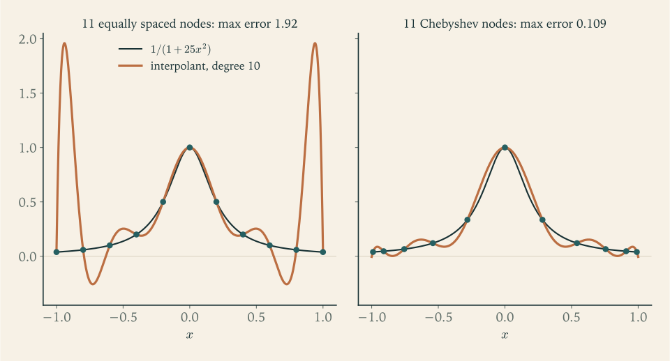
Figure 4.1 shows where the error lives. With equally spaced nodes the interpolant is excellent in the middle of the interval and useless near the ends. With Chebyshev nodes there is no such blow-up: the error is moderate everywhere and largest near the centre, where the function itself changes fastest.
4.5 Sensitivity to the data: the Lebesgue constant
So far the data were exact. Measured or rounded data carry errors, and the interpolant inherits them. How much are they magnified?
Definition 4.7 (Lebesgue constant). For nodes \(x_0,\dots,x_n\) in \([a,b]\) with Lagrange basis \(\ell_0,\dots,\ell_n\) , the Lebesgue constant is
Theorem 4.8 (stability and near-best approximation). Let \(p\) interpolate \(f\) at the given nodes. (a) If \(\tilde p\) interpolates perturbed values \(\tilde y_j\) with \(\lvert\tilde y_j-f(x_j)\rvert\le\epsilon\) for all \(j\) , then \(\lVert p-\tilde p\rVert_\infty\le\Lambda_n\,\epsilon\) , and some perturbation of that size attains equality. (b) For every \(q\in\mathcal P_n\) ,
Proof. (a) \(p-\tilde p=\sum_j(f(x_j)-\tilde y_j)\,\ell_j\) , so \(\lvert p(x)-\tilde p(x)\rvert\le\epsilon\sum_j\lvert\ell_j(x)\rvert\le\epsilon\Lambda_n\) . For equality let \(x^\star\) be a point where the sum is largest and take \(\tilde y_j=f(x_j)-\epsilon\operatorname{sign}\ell_j(x^\star)\) . (b) Interpolation is linear in the data and reproduces every polynomial of degree at most \(n\) , so \(p-q\) is the interpolant of the function \(f-q\) , whose values at the nodes are at most \(\lVert f-q\rVert_\infty\) in magnitude. By (a), \(\lVert p-q\rVert_\infty\le\Lambda_n\lVert f-q\rVert_\infty\) , and \(\lVert f-p\rVert_\infty\le\lVert f-q\rVert_\infty+\lVert q-p\rVert_\infty\) .
Part (a) says that \(\Lambda_n\) is the condition number, in the absolute sense, of the map from data to interpolant. Part (b) says the interpolant is within a factor \(1+\Lambda_n\) of the best that any polynomial of the same degree could do. Everything therefore hinges on the size of \(\Lambda_n\) , and that depends only on the nodes. For equally spaced nodes it grows exponentially, roughly like \(2^{n+1}/(e\,n\ln n)\) . For Chebyshev nodes it grows only logarithmically, staying below \(\tfrac2\pi\ln(n+1)+1\) . We state these growth rates without proof and check them numerically.
Example 4.5: Lebesgue constants and a worst-case perturbation
Computing \(\max\sum_j\lvert\ell_j(x)\rvert\) on a fine grid of \([-1,1]\) gives:
| \(n\) | \(\Lambda_n\) , equally spaced | \(\Lambda_n\) , Chebyshev | \(\tfrac2\pi\ln(n+1)+1\) |
|---|---|---|---|
| \(5\) | \(3.11\) | \(2.10\) | \(2.14\) |
| \(10\) | \(29.9\) | \(2.49\) | \(2.53\) |
| \(20\) | \(1.10\times10^{4}\) | \(2.90\) | \(2.94\) |
| \(30\) | \(6.60\times10^{6}\) | \(3.15\) | \(3.19\) |
To see what this means, interpolate \(e^{x}\) on \([-1,1]\) with \(n=20\) . The truncation error is negligible for both node sets, because all derivatives of \(e^{x}\) are bounded by \(e\) : Corollary 4.5 bounds it by \(e\,\lVert\omega\rVert_\infty/21!\) , which is \(1.2\times10^{-23}\) for equally spaced nodes and smaller still for Chebyshev nodes. Yet the computed interpolant on equally spaced nodes is in error by a few times \(10^{-12}\) , while on Chebyshev nodes it is accurate to about \(2\times10^{-15}\) . No data were perturbed on purpose. The data are the double-precision values of \(e^{x_j}\) , each carrying a relative rounding error of order \(u\) , and the equally spaced interpolant has magnified those errors by a factor of order \(\Lambda_{20}\) : indeed \(\Lambda_{20}\,u\,e=3\times10^{-12}\) . Now perturb each data value deliberately by \(\pm10^{-6}\) , with the signs of the worst case of Theorem 4.8(a). The equally spaced interpolant moves by \(1.10\times10^{-2}\) , which is \(\Lambda_{20}\times10^{-6}\) : data good to six digits yield an interpolant good to two. The Chebyshev interpolant moves by \(2.9\times10^{-6}\) .
So high-degree interpolation at equally spaced points fails twice over. For some functions the truncation error diverges, and for all functions the problem is ill conditioned: data errors, including the rounding errors of Chapter 1, are amplified exponentially. At \(n=65\) the amplification factor exceeds \(1/u\) , and even exact data stored in double precision produce garbage.
Common mistake. Assuming that a polynomial through more data points is a better approximation, or trusting an interpolant outside the range of its nodes. Between widely separated or equally spaced nodes a high-degree interpolant can oscillate with an amplitude unrelated to the data, and outside the interval \(\lvert\omega(x)\rvert\) grows like the \((n+1)\) -st power of the distance, so extrapolation is far worse than interpolation. If the nodes can be chosen, use Chebyshev nodes. If they cannot, because the data come from equally spaced measurements, do not raise the degree; use the piecewise polynomials of Chapter 5.
For evaluating the interpolant, the formula to use in practice is the barycentric formula. With weights \(w_j=1/\prod_{m\ne j}(x_j-x_m)\) the Lagrange basis is \(\ell_j(x)=\omega(x)\,w_j/(x-x_j)\) , and dividing \(p=\sum y_j\ell_j\) by the identity \(1=\sum\ell_j\) cancels \(\omega\) :
After a one-time cost proportional to \(n^2\) for the weights, each evaluation costs a number of operations proportional to \(n\) , and for Chebyshev nodes the formula is numerically stable for \(n\) in the thousands. Every interpolant in this chapter was evaluated this way.
4.6 Matching derivatives
Sometimes the data include slopes. Hermite interpolation asks for a polynomial that matches \(f\) and \(f'\) at each node. The case needed later is the cubic on a single interval: given values \(f_0,f_1\) and slopes \(d_0,d_1\) at the ends of \([x_0,x_1]\) with \(h=x_1-x_0\) and \(t=(x-x_0)/h\) , the unique cubic with those four data is
as one verifies by checking the four conditions. Its error has the form of Theorem 4.4 with each node counted twice: for \(f\) with four continuous derivatives,
The proof repeats the Rolle argument, with \(\varphi(t)=f(t)-H(t)-K(t-x_0)^2(t-x_1)^2\) having double zeros at the two nodes.
Example 4.6: A Hermite cubic for the exponential
For \(f(x)=e^{x}\) on \([0,1]\) the data are \(f_0=d_0=1\) and \(f_1=d_1=e\) . At the midpoint \(t=\tfrac12\) the four basis values are \(\tfrac12\) , \(\tfrac18\) , \(\tfrac12\) , \(-\tfrac18\) , so
The exact value is \(e^{0.5}=1.648721\) , an error of \(4.37\times10^{-3}\) . The error formula gives \(f''''(\xi)\,(0.5)^2(0.5)^2/24=e^{\xi}/384\) for some \(\xi\in(0,1)\) , hence a value between \(1/384=2.60\times10^{-3}\) and \(e/384=7.08\times10^{-3}\) . The observed error corresponds to \(\xi=0.52\) .
A cubic that matches values and slopes at both ends of an interval can be joined to its neighbours without a corner. That is the idea of the next chapter. High-degree polynomials on a whole interval are powerful when the nodes are free and the function is smooth, and treacherous otherwise; a theorem of Weierstrass guarantees that every continuous function on \([a,b]\) can be approximated uniformly by polynomials, yet for any fixed scheme of nodes there are continuous functions whose interpolants fail to converge. Low-degree pieces, joined smoothly, converge for every reasonable function and every reasonable set of nodes. And when the data are noisy, passing a curve exactly through them is itself the mistake, which leads to least squares.
Exercises
-
Write the Lagrange basis for the nodes \(-1,0,2\) , use it to find the polynomial of degree at most \(2\) through \((-1,2)\) , \((0,1)\) , \((2,5)\) , simplify it, and evaluate it at \(x=1\) .
Answer
\(\ell_0(x)=x(x-2)/3\) , \(\ell_1(x)=-(x+1)(x-2)/2\) , \(\ell_2(x)=x(x+1)/6\) , and \(p=2\ell_0+\ell_1+5\ell_2=x^2+1\) , so \(p(1)=2\) .
-
Let \(\ell_0,\dots,\ell_n\) be the Lagrange basis for distinct nodes \(x_0,\dots,x_n\) . Prove that \(\sum_j\ell_j(x)=1\) and, more generally, \(\sum_jx_j^{k}\ell_j(x)=x^{k}\) for \(k=0,1,\dots,n\) , and explain why the identity fails for \(k=n+1\) .
Solution
Fix \(k\) with \(0\le k\le n\) and consider the function \(f(x)=x^{k}\) . It is a polynomial of degree at most \(n\) , and it takes the values \(x_j^{k}\) at the nodes. The Lagrange form of the interpolant of these data is \(p(x)=\sum_jx_j^{k}\ell_j(x)\) , which also lies in \(\mathcal P_n\) and takes the same values at the nodes. By the uniqueness part of Theorem 4.1 there is only one such polynomial, so \(p=f\) , that is, \(\sum_jx_j^{k}\ell_j(x)=x^{k}\) for every real \(x\) . The case \(k=0\) is \(\sum_j\ell_j(x)=1\) .
For \(k=n+1\) the argument breaks at its first step: \(x^{n+1}\) is not in \(\mathcal P_n\) , so uniqueness within \(\mathcal P_n\) says nothing about it. In fact \(q(x)=x^{n+1}-\sum_jx_j^{n+1}\ell_j(x)\) is a monic polynomial of degree \(n+1\) that vanishes at all \(n+1\) nodes, so \(q=\omega\) , the node polynomial, and the identity fails by exactly \(\omega(x)\) . This is Theorem 4.4 for \(f(x)=x^{n+1}\) , whose \((n+1)\) -st derivative is the constant \((n+1)!\) .
-
Build the divided-difference table for the data \((1,2)\) , \((2,3)\) , \((4,11)\) , \((5,18)\) , write the interpolant in Newton form, evaluate it at \(x=3\) , and explain what the value of the third divided difference tells you about the data.
Solution
The columns of the table are computed from the recursion of Theorem 4.3.
\(x_i\) \(f[x_i]\) first second third \(1\) \(2\) \(1\) \(1\) \(0\) \(2\) \(3\) \(4\) \(1\) \(4\) \(11\) \(7\) \(5\) \(18\) First differences: \((3-2)/(2-1)=1\) , \((11-3)/(4-2)=4\) , \((18-11)/(5-4)=7\) . Second differences: \((4-1)/(4-1)=1\) and \((7-4)/(5-2)=1\) . Third difference: \((1-1)/(5-1)=0\) . The Newton form uses the top entries:
\[ p(x)=2+1\cdot(x-1)+1\cdot(x-1)(x-2)+0\cdot(x-1)(x-2)(x-4). \]At \(x=3\) this gives \(p(3)=2+2+2=6\) . Expanding, \(p(x)=x^2-2x+3\) .
The third divided difference is zero, so the cubic term is absent: the four data points lie on a single quadratic. By Corollary 4.5 a divided difference of order three equals \(f'''(\eta)/6\) for a smooth underlying function, so a vanishing third difference is what one expects when the data are generated by a polynomial of degree two, and one can confirm that \(x^2-2x+3\) reproduces all four values.
-
A fifth point \((3,7)\) is added to the data of Exercise 4.3. Extend the table by one diagonal, give the new Newton coefficient, and write the new interpolant as the old one plus a single term.
Answer
The new diagonal, from the bottom of each column, is \(7\) , \(\tfrac{11}2\) , \(\tfrac32\) , \(\tfrac12\) , \(\tfrac14\) : for instance \(f[5,3]=(7-18)/(3-5)=\tfrac{11}2\) and \(f[4,5,3]=(\tfrac{11}2-7)/(3-4)=\tfrac32\) . The new coefficient is \(\tfrac14\) , and \(p_4(x)=p_3(x)+\tfrac14(x-1)(x-2)(x-4)(x-5)\) . Check: \(p_4(3)=6+\tfrac14(2)(1)(-1)(-2)=7\) .
-
For \(f(x)=1/x\) and distinct positive nodes, prove by induction on \(n\) , using the recursion of Theorem 4.3, that \(f[x_0,\dots,x_n]=(-1)^{n}/(x_0x_1\cdots x_n)\) , and check the formula against Corollary 4.5.
Solution
Base case. For \(n=0\) , \(f[x_0]=f(x_0)=1/x_0=(-1)^{0}/x_0\) .
Inductive step. Suppose the formula holds for every set of \(n\) distinct positive nodes. By the recursion of Theorem 4.3 and the inductive hypothesis applied to \(x_1,\dots,x_n\) and to \(x_0,\dots,x_{n-1}\) ,
\[ f[x_0,\dots,x_n]=\frac{1}{x_n-x_0}\left(\frac{(-1)^{n-1}}{x_1\cdots x_n}-\frac{(-1)^{n-1}}{x_0\cdots x_{n-1}}\right) =\frac{(-1)^{n-1}}{x_n-x_0}\cdot\frac{x_0-x_n}{x_0x_1\cdots x_n}=\frac{(-1)^{n}}{x_0x_1\cdots x_n}, \]where the two fractions were put over the common denominator \(x_0x_1\cdots x_n\) . This completes the induction.
Check against Corollary 4.5. For \(f(x)=1/x\) , \(f^{(n)}(x)=(-1)^{n}n!/x^{n+1}\) , so the corollary asserts \(f[x_0,\dots,x_n]=(-1)^{n}/\eta^{n+1}\) for some \(\eta\) between the smallest and largest node. Comparing with the formula just proved, \(\eta^{n+1}=x_0x_1\cdots x_n\) : the point \(\eta\) is the geometric mean of the nodes, which does lie between the smallest and the largest. For the nodes \(1,2,4\) the formula gives \(f[1,2,4]=1/8\) , and \(\eta=2\) .
-
Interpolate \(e^{x}\) at the nodes \(0\) , \(0.5\) , \(1\) by a quadratic. Use Theorem 4.4 to give upper and lower bounds for the error at \(x=0.25\) , compare with the actual error, and bound the error over the whole interval.
Solution
Here \(n=2\) and \(f'''(x)=e^{x}\) , so Theorem 4.4 gives \(f(x)-p(x)=e^{\xi}\,\omega(x)/6\) with \(\xi\in(0,1)\) . At \(x=0.25\) ,
\[ \omega(0.25)=(0.25)(0.25-0.5)(0.25-1)=0.046875>0 . \]Since \(1<e^{\xi}<e\) , the error is positive and lies between \(0.046875/6\) and \(e\times0.046875/6\) , that is, between \(7.81\times10^{-3}\) and \(2.12\times10^{-2}\) .
The actual interpolant is \(p(0.25)=1.271756\) and \(e^{0.25}=1.284025\) , so the error is \(1.227\times10^{-2}\) , inside the predicted range; it corresponds to \(e^{\xi}=1.57\) , that is, \(\xi=0.45\) .
Over the whole interval, the three nodes are equally spaced with \(h=0.5\) , so by Exercise 4.8 \(\lVert\omega\rVert_\infty=2h^3/(3\sqrt3)=0.0481\) , and Corollary 4.5 gives \(\lVert f-p\rVert_\infty\le e\times0.0481/6=2.18\times10^{-2}\) . The largest actual error on a fine grid is \(1.44\times10^{-2}\) . The bound overestimates by about half because it pairs the largest value of \(e^{\xi}\) with the largest value of \(\lvert\omega\rvert\) , which need not occur together.
-
A table of \(\ln x\) on \([1,2]\) is to be used with linear interpolation. Find the largest spacing \(h\) that guarantees an interpolation error below \(10^{-6}\) , and the largest spacing if quadratic interpolation through three consecutive entries is used, given that \(\max\lvert(x-x_0)(x-x_1)(x-x_2)\rvert=2h^3/(3\sqrt3)\) for equally spaced nodes.
Answer
Linear: \(\lvert f''(x)\rvert=1/x^2\le1\) on \([1,2]\) , so \(h^2/8\le10^{-6}\) gives \(h\le2.83\times10^{-3}\) . Quadratic: \(\lvert f'''(x)\rvert=2/x^3\le2\) , so the error is at most \(\tfrac26\cdot2h^3/(3\sqrt3)=2h^3/(9\sqrt3)\) , and requiring this to be at most \(10^{-6}\) gives \(h\le0.0198\) . The quadratic rule needs a table seven times shorter.
-
Prove that \(\max\lvert(x-x_0)(x-x_1)\rvert\) over \([x_0,x_1]\) is \(h^2/4\) with \(h=x_1-x_0\) , and that for three equally spaced nodes with spacing \(h\) the maximum of \(\lvert\omega\rvert\) over \([x_0,x_2]\) is \(2h^3/(3\sqrt3)\) .
Solution
Two nodes. On \([x_0,x_1]\) write \(x=x_0+s\) with \(0\le s\le h\) . Then \(\lvert(x-x_0)(x-x_1)\rvert=s(h-s)\) , a downward parabola in \(s\) with zeros at \(0\) and \(h\) and maximum at the midpoint \(s=h/2\) , where it equals \(h^2/4\) .
Three nodes. Place the origin at the middle node, so the nodes are \(-h,0,h\) and \(\omega(x)=(x+h)\,x\,(x-h)=x^3-h^2x\) . On \([-h,h]\) the function \(\omega\) vanishes at the endpoints and at \(0\) , so the maximum of \(\lvert\omega\rvert\) occurs at an interior critical point. Setting \(\omega'(x)=3x^2-h^2=0\) gives \(x=\pm h/\sqrt3\) , and
\[ \Bigl\lvert\omega\bigl(h/\sqrt3\bigr)\Bigr\rvert=\frac{h}{\sqrt3}\Bigl(h^2-\frac{h^2}{3}\Bigr)=\frac{h}{\sqrt3}\cdot\frac{2h^2}{3}=\frac{2h^3}{3\sqrt3}. \]By symmetry the value at \(-h/\sqrt3\) has the same magnitude. These are the only critical points, so \(\max\lvert\omega\rvert=2h^3/(3\sqrt3)\approx0.385h^3\) , attained at a distance \(0.577h\) on either side of the middle node.
-
Use the recurrence to compute \(T_4\) , list its zeros, and confirm that the monic polynomial \(\tfrac18T_4\) has maximum norm \(\tfrac18\) on \([-1,1]\) ; then compute the maximum norm of the monic quartic whose zeros are the equally spaced points \(-1,-\tfrac13,\tfrac13,1\) and compare.
Answer
\(T_2=2x^2-1\) , \(T_3=4x^3-3x\) , \(T_4=2xT_3-T_2=8x^4-8x^2+1\) . Its zeros are \(\pm\cos(\pi/8)=\pm0.9239\) and \(\pm\cos(3\pi/8)=\pm0.3827\) . Since \(\lvert T_4\rvert\le1\) with equality at \(0,\pm1/\sqrt2,\pm1\) , the monic polynomial \(\tfrac18T_4=x^4-x^2+\tfrac18\) has norm \(\tfrac18=0.125\) . The quartic with zeros \(\pm1,\pm\tfrac13\) is \((x^2-1)(x^2-\tfrac19)\) ; as a function of \(s=x^2\) it is smallest at \(s=\tfrac59\) , where it equals \(-\tfrac{16}{81}\) , so its norm is \(\tfrac{16}{81}=0.198\) , about \(58\) percent larger.
-
Interpolate \(e^{x}\) on \([0,2]\) by a quartic at the five Chebyshev nodes mapped to that interval. Give the nodes, the value of \(\lVert\omega\rVert_\infty\) , and the resulting error bound, and say how the bound would change for five equally spaced nodes, for which \(\lVert\omega\rVert_\infty=0.1135\) .
Solution
The Chebyshev nodes for \(n=4\) on \([-1,1]\) are \(\cos\bigl((2j+1)\pi/10\bigr)\) , \(j=0,\dots,4\) , and the map \(x\mapsto1+x\) carries \([-1,1]\) onto \([0,2]\) . The mapped nodes are \(1.9511\) , \(1.5878\) , \(1\) , \(0.4122\) , \(0.0489\) .
On \([a,b]\) the node polynomial of the mapped Chebyshev nodes has \(\lVert\omega\rVert_\infty=2\bigl((b-a)/4\bigr)^{n+1}\) . With \(b-a=2\) and \(n=4\) this is \(2\,(0.5)^5=0.0625\) . The fifth derivative of \(e^{x}\) is \(e^{x}\) , with maximum \(e^2\) on \([0,2]\) . Corollary 4.5 gives
\[ \lVert f-p\rVert_\infty\le\frac{e^2}{5!}\times0.0625=3.85\times10^{-3}. \]The actual maximum error of this interpolant on a fine grid is \(1.74\times10^{-3}\) , under the bound.
For five equally spaced nodes \(0,0.5,1,1.5,2\) the only change is \(\lVert\omega\rVert_\infty=0.1135\) , so the bound becomes \(e^2\times0.1135/120=6.99\times10^{-3}\) , larger by the ratio \(0.1135/0.0625=1.8\) . At this low degree the advantage of Chebyshev nodes is modest; by Theorem 4.6 it grows geometrically with \(n\) .
-
A student fits the polynomial of degree \(11\) through population counts at twelve equally spaced census years and uses it to predict the population ten years after the last census. Explain, using \(\omega\) and the Lebesgue constant, two separate reasons to distrust the prediction, and suggest what to do instead.
Hint
First reason: the prediction point lies outside the interval of the nodes; estimate how large \(\lvert\omega(x)\rvert\) is one spacing beyond the last of twelve equally spaced nodes compared with its size between them. Second reason: census counts carry errors, and \(\Lambda_{11}\) for equally spaced nodes is already about \(50\) inside the interval and far larger outside. A low-degree model fitted by least squares (Chapter 5) through the last few censuses is the defensible alternative.
-
Compute the Lebesgue constant for the three equally spaced nodes \(-1,0,1\) on \([-1,1]\) by finding \(\sum_j\lvert\ell_j(x)\rvert\) explicitly on \([0,1]\) , and say what it implies about quadratic interpolation of data known to within \(\epsilon\) .
Solution
For the nodes \(-1,0,1\) the Lagrange basis is
\[ \ell_0(x)=\tfrac12x(x-1),\qquad\ell_1(x)=1-x^2,\qquad\ell_2(x)=\tfrac12x(x+1). \]On \([0,1]\) we have \(x(x-1)\le0\) , \(1-x^2\ge0\) , and \(x(x+1)\ge0\) , so
\[ \sum_j\lvert\ell_j(x)\rvert=-\tfrac12x(x-1)+(1-x^2)+\tfrac12x(x+1)=1+x-x^2 . \]This is \(1+x-x^2\) , a downward parabola with maximum at \(x=\tfrac12\) , where it equals \(\tfrac54\) . The Lebesgue function is even, because the node set is symmetric about \(0\) , so the same maximum occurs on \([-1,0]\) at \(x=-\tfrac12\) . Hence \(\Lambda_2=\tfrac54\) .
By Theorem 4.8(a), if each of the three data values is known to within \(\epsilon\) , the quadratic interpolant is determined to within \(1.25\,\epsilon\) everywhere on \([-1,1]\) : interpolation at three equally spaced points amplifies data errors by at most a quarter. By part (b), it is within a factor \(2.25\) of the best quadratic approximation.
-
In Theorem 4.8(a), verify in detail that the perturbation \(\tilde y_j=f(x_j)-\epsilon\operatorname{sign}\ell_j(x^\star)\) gives \(\lvert p(x^\star)-\tilde p(x^\star)\rvert=\Lambda_n\epsilon\) , and explain why a random perturbation of the same size typically produces a much smaller change.
Hint
Substitute the perturbation into \(p(x^\star)-\tilde p(x^\star)=\sum_j(f(x_j)-\tilde y_j)\ell_j(x^\star)\) and use \(\operatorname{sign}(a)\,a=\lvert a\rvert\) . For the second part note that the worst case needs all \(n+1\) signs to match those of \(\ell_j(x^\star)\) ; with random signs the terms partly cancel, and the typical size is \(\epsilon\bigl(\sum_j\ell_j(x)^2\bigr)^{1/2}\) instead of \(\epsilon\sum_j\lvert\ell_j(x)\rvert\) .
-
Compute the barycentric weights for the nodes \(0,1,3\) and use the barycentric formula to evaluate at \(x=2\) the interpolant of the data of Example 4.1, confirming the value found there.
Solution
The weights are \(w_j=1/\prod_{m\ne j}(x_j-x_m)\) :
\[ w_0=\tfrac13,\quad w_1=-\tfrac12,\quad w_2=\tfrac16, \]from \((0-1)(0-3)=3\) , \((1-0)(1-3)=-2\) , and \((3-0)(3-1)=6\) . At \(x=2\) the differences \(x-x_j\) are \(2\) , \(1\) , \(-1\) , so the terms \(w_j/(x-x_j)\) are \(\tfrac16\) , \(-\tfrac12\) , \(-\tfrac16\) . With the data \(y=(1,3,2)\) ,
\[ \text{numerator}=\tfrac16(1)-\tfrac12(3)-\tfrac16(2)=-\tfrac53,\qquad\text{denominator}=\tfrac16-\tfrac12-\tfrac16=-\tfrac12 , \]and the quotient is \((-\tfrac53)/(-\tfrac12)=\tfrac{10}3\) , the value found in Example 4.1. The barycentric formula never forms the polynomial’s coefficients or the node polynomial; once the weights are known, each evaluation is two short sums and a division, and changing the data \(y_j\) requires no new setup at all.
-
The Vandermonde matrix for \(n+1\) equally spaced nodes on \([-1,1]\) has condition number about \(1.4\times10^{4}\) for \(n=10\) and \(8.3\times10^{8}\) for \(n=20\) in the \(2\) -norm. Using the ideas of Chapter 1, estimate how many digits of the monomial coefficients survive in double precision in each case, and explain why this does not by itself mean the interpolant is inaccurate.
Answer
By the rule of Chapter 1 a backward stable solver loses about \(\log_{10}\kappa\) digits: roughly \(4\) of \(16\) for \(n=10\) , leaving \(12\) , and roughly \(9\) for \(n=20\) , leaving \(7\) . But the quantity of interest is the interpolant, not its monomial coefficients. A backward stable solve returns coefficients that reproduce slightly perturbed data, so the computed polynomial still nearly interpolates; its accuracy as a function is governed by \(\Lambda_n\) and by cancellation in evaluating the monomial sum, not by \(\kappa\) of the Vandermonde matrix alone.
-
Expand \(f(x)=1/(1+25x^2)\) as a geometric series to show that \(f^{(n)}(0)=(-1)^{n/2}\,n!\,5^{n}\) for even \(n\) , and explain how this growth, combined with Corollary 4.5, makes the divergence in Example 4.4 plausible.
Hint
For \(\lvert x\rvert<\tfrac15\) , \(1/(1+25x^2)=\sum_k(-25x^2)^{k}\) ; read off the coefficient of \(x^{n}\) and compare with \(f^{(n)}(0)/n!\) . Then \(\lVert f^{(n+1)}\rVert_\infty/(n+1)!\) is at least of order \(5^{n+1}\) , while \(\lVert\omega\rVert_\infty\) for equally spaced nodes in Example 4.4 shrinks only by a factor of about \(1.4\) per unit increase in \(n\) .
-
Find the cubic \(H\) with \(H(0)=0\) , \(H'(0)=1\) , \(H(1)=1\) , \(H'(1)=0\) using the formula of Section 4.6, and verify the four conditions directly.
Answer
With \(h=1\) , \(f_0=0\) , \(d_0=1\) , \(f_1=1\) , \(d_1=0\) : \(H(x)=(x^3-2x^2+x)+(-2x^3+3x^2)=-x^3+x^2+x\) . Then \(H(0)=0\) , \(H(1)=1\) , and \(H'(x)=-3x^2+2x+1\) gives \(H'(0)=1\) , \(H'(1)=0\) .
-
Inverse interpolation. For \(f(x)=x^3-2x-5\) the values at \(x=2,\,2.1,\,2.2\) are \(-1\) , \(0.061\) , \(1.248\) . Regard \(x\) as a function of \(y=f(x)\) , build the divided-difference table of \(x\) against \(y\) , and evaluate the quadratic at \(y=0\) to estimate the root; compare its error with that of the secant step from the first two points.
Solution
Treat the \(y\) -values \(-1\) , \(0.061\) , \(1.248\) as the nodes and the \(x\) -values \(2\) , \(2.1\) , \(2.2\) as the data. The first divided differences are
\[ \frac{2.1-2}{0.061-(-1)}=0.0942507,\qquad\frac{2.2-2.1}{1.248-0.061}=0.0842460, \]and the second is \((0.0842460-0.0942507)/(1.248-(-1))=-0.00445049\) . The Newton form of the quadratic \(q(y)\) interpolating \(x\) as a function of \(y\) is
\[ q(y)=2+0.0942507\,(y+1)-0.00445049\,(y+1)(y-0.061), \]and the root estimate is its value at \(y=0\) :
\[ q(0)=2+0.0942507+0.00445049\times0.061=2.0945222 . \]The true root is \(2.0945515\) , so the error is \(-2.93\times10^{-5}\) . The secant step from the first two points is the linear inverse interpolant evaluated at \(0\) , namely \(2+0.0942507=2.0942507\) , with error \(-3.01\times10^{-4}\) . One extra function value, used through a quadratic in \(y\) , improves the estimate tenfold. This inverse quadratic step is the fast step in Brent’s method; it requires the three \(y\) -values to be distinct, and it is trusted only when the result stays inside the current bracket.
-
Let \(f''>0\) on \([x_0,x_1]\) . Use Theorem 4.4 to show that the linear interpolant lies above \(f\) strictly between the nodes, and state the corresponding result for extrapolation just outside the interval.
Hint
With \(n=1\) the error is \(\tfrac12f''(\xi)(x-x_0)(x-x_1)\) . Determine the sign of the product \((x-x_0)(x-x_1)\) for \(x\) between the nodes and for \(x\) just outside them.
-
Table values are rounded to five decimal places, so each carries an error of at most \(5\times10^{-6}\) . Bound the effect of this rounding on the interpolated value for linear interpolation between adjacent entries and for the degree-\(10\) interpolant through eleven equally spaced entries, using the Lebesgue constants of Section 4.5.
Answer
Linear interpolation between two adjacent entries has \(\Lambda_1=1\) , so the rounding contributes at most \(5\times10^{-6}\) . For eleven equally spaced nodes \(\Lambda_{10}=29.9\) , so the contribution can reach \(29.9\times5\times10^{-6}=1.5\times10^{-4}\) : the high-degree interpolant can turn five-decimal data into values wrong in the fourth decimal.