Chapter 4 ended with two warnings. A single high-degree polynomial through equally spaced data oscillates, and no interpolant of any kind should be passed through data that contain noise. Both warnings describe everyday situations. Measurements arrive on a uniform grid whether we like it or not: a sensor samples every second, a census is taken every ten years, and the nodes cannot be moved to Chebyshev positions after the fact. And measurements are never exact.
This chapter gives the two standard answers. When the data are trustworthy and equally spaced, use many polynomials of low degree, one per subinterval, joined so that the result is smooth; the cubic spline is the outcome, and it converges for every smooth function on every reasonable grid. When the data are noisy, give up on reproducing them and look for the simplest function that comes closest to all of them at once; that is the least-squares fit. The second answer raises a numerical question that the first does not. The obvious way to compute a least-squares fit squares the condition number of the problem, and a better algorithm avoids the squaring. That contrast, between a formula that is correct and an algorithm that is stable, is a small-scale rehearsal for the treatment of linear systems in Chapter 7.
5.1 Many short pieces instead of one long polynomial
Fix knots \(a=x_0<x_1<\dots<x_n=b\) and let \(h=\max_i(x_{i+1}-x_i)\) . The simplest piecewise interpolant joins consecutive data points by straight lines. On each subinterval it is the linear interpolant of Section 4.3, whose error is at most \(\tfrac18(x_{i+1}-x_i)^2\max\lvert f''\rvert\) , so over the whole interval:
Proposition 5.1 (piecewise linear interpolation). If \(f\) is twice continuously differentiable on \([a,b]\) and \(s\) is the piecewise linear interpolant of \(f\) at the knots, then
The contrast with Chapter 4 is that the bound involves a fixed derivative, the second, however many knots there are. Refining the grid can only help: halving \(h\) divides the bound by four. There is no Runge phenomenon, because the degree never rises.
Example 5.1: The Runge function tamed by straight lines
For \(f(x)=1/(1+25x^2)\) on \([-1,1]\) the second derivative is largest at the origin, where \(\lvert f''(0)\rvert=50\) . With \(n\) equal subintervals \(h=2/n\) , and the maximum errors of the piecewise linear interpolant on a fine grid are:
| \(n\) | \(10\) | \(20\) | \(40\) | \(80\) | \(160\) |
|---|---|---|---|---|---|
| error | \(6.74\times10^{-2}\) | \(4.18\times10^{-2}\) | \(1.40\times10^{-2}\) | \(3.80\times10^{-3}\) | \(9.70\times10^{-4}\) |
| bound \(50h^2/8\) | \(2.50\times10^{-1}\) | \(6.25\times10^{-2}\) | \(1.56\times10^{-2}\) | \(3.91\times10^{-3}\) | \(9.77\times10^{-4}\) |
Once the grid resolves the central peak, each doubling of \(n\) divides the error by nearly four, and the error approaches the bound from below. The proposition also answers a design question before any computation: for an error below \(10^{-3}\) it suffices that \(50h^2/8\le10^{-3}\) , that is, \(n\ge2/\sqrt{8\times10^{-3}/50}=158.1\) , so \(159\) subintervals. With \(n=159\) the observed error is \(9.88\times10^{-4}\) .
The price of this safety is roughness. The piecewise linear interpolant has a corner at every knot, and \(160\) pieces were needed for three digits. Raising the degree of the pieces to three allows the corners to be removed and the accuracy to improve from \(h^2\) to \(h^4\) .
5.2 Cubic splines
Definition 5.2 (cubic spline interpolant). Given knots \(x_0<\dots<x_n\) and values \(y_0,\dots,y_n\) , a cubic spline interpolant is a function \(s\) on \([x_0,x_n]\) such that \(s\) is a cubic polynomial on each subinterval \([x_i,x_{i+1}]\) , \(s(x_i)=y_i\) for all \(i\) , and \(s\) , \(s'\) , and \(s''\) are continuous on \([x_0,x_n]\) .
Count the freedoms. There are \(n\) cubics with \(4n\) coefficients. Interpolation at both ends of each piece gives \(2n\) conditions, which also make \(s\) continuous. Continuity of \(s'\) and of \(s''\) at the \(n-1\) interior knots gives \(2(n-1)\) more. That is \(4n-2\) conditions for \(4n\) unknowns, so two further conditions are needed, and they are imposed at the ends. The natural spline sets \(s''(x_0)=s''(x_n)=0\) . The clamped or complete spline prescribes the end slopes, \(s'(x_0)=f'(x_0)\) and \(s'(x_n)=f'(x_n)\) . The not-a-knot spline, the default in most software, requires \(s'''\) to be continuous at \(x_1\) and at \(x_{n-1}\) , so that the first two and the last two pieces are each a single cubic; it needs no information beyond the data.
The efficient way to compute a spline is to take as unknowns the second derivatives \(M_i=s''(x_i)\) at the knots. Write \(h_i=x_{i+1}-x_i\) and \(\delta_i=(y_{i+1}-y_i)/h_i\) for the slope of the data on the \(i\) -th subinterval. Since \(s\) is cubic on \([x_i,x_{i+1}]\) , \(s''\) is linear there and is determined by its end values \(M_i\) and \(M_{i+1}\) . Integrating twice and choosing the two constants of integration to satisfy \(s(x_i)=y_i\) and \(s(x_{i+1})=y_{i+1}\) gives, for \(x_i\le x\le x_{i+1}\) ,
By construction \(s\) and \(s''\) are continuous whatever the \(M_i\) are. Continuity of \(s'\) is what determines them. Differentiating the formula on \([x_i,x_{i+1}]\) and on \([x_{i-1},x_i]\) and equating the two values at \(x_i\) gives, after collecting terms,
With the natural conditions \(M_0=M_n=0\) this is a system of \(n-1\) linear equations in \(M_1,\dots,M_{n-1}\) whose matrix is tridiagonal: each equation involves only three consecutive unknowns. Whether it can be solved is settled by a property of the matrix.
Lemma 5.3 (strict diagonal dominance implies nonsingularity). Let \(A\) be an \(n\times n\) matrix with \(\lvert a_{kk}\rvert>\sum_{j\ne k}\lvert a_{kj}\rvert\) for every row \(k\) . Then \(A\) is nonsingular.
Proof. Suppose \(Az=0\) with \(z\ne0\) , and let \(k\) be an index with \(\lvert z_k\rvert=\max_j\lvert z_j\rvert>0\) . Row \(k\) of \(Az=0\) reads \(a_{kk}z_k=-\sum_{j\ne k}a_{kj}z_j\) , so \(\lvert a_{kk}\rvert\lvert z_k\rvert\le\sum_{j\ne k}\lvert a_{kj}\rvert\lvert z_j\rvert\le\lvert z_k\rvert\sum_{j\ne k}\lvert a_{kj}\rvert<\lvert a_{kk}\rvert\lvert z_k\rvert\) , a contradiction.
Theorem 5.4 (existence and uniqueness of the natural cubic spline). For any knots \(x_0<\dots<x_n\) and any values \(y_0,\dots,y_n\) there is exactly one natural cubic spline interpolant.
Proof. In row \(i\) of the system for \(M_1,\dots,M_{n-1}\) the diagonal entry is \(2(h_{i-1}+h_i)\) and the off-diagonal entries are \(h_{i-1}\) and \(h_i\) (one of them absent in the first and last rows), with sum at most \(h_{i-1}+h_i\) . The matrix is strictly diagonally dominant, hence nonsingular by Lemma 5.3, so the \(M_i\) exist and are unique. Every natural spline interpolant arises from its values of \(s''\) at the knots through the displayed formula, and those values must satisfy the system; so the spline is unique, and the formula with the solution \(M_i\) shows that it exists.
The same argument, with two extra equations for the end conditions, handles the clamped spline. A tridiagonal system is solved by elimination in a number of operations proportional to \(n\) (Section 7.5), so a spline through a million points costs a few million operations. A polynomial interpolant through a million points is not even a meaningful object.
Example 5.2: A natural spline through four points
Take the knots \(0,1,2,3\) with values \(1,3,2,5\) . Here every \(h_i=1\) , the data slopes are \(\delta_0=2\) , \(\delta_1=-1\) , \(\delta_2=3\) , and the two equations are
Subtracting four times the second from the first gives \(-15M_2=-114\) , so \(M_2=7.6\) and \(M_1=-6.4\) ; and \(M_0=M_3=0\) . On the middle interval \([1,2]\) the formula of this section reads
and at the midpoint \(s(1.5)=\tfrac{1.2}{6}(0.125)+4.0667(0.5)+0.7333(0.5)=2.425\) . The slopes at the knots come out as \(s'(0)=3.0667\) , \(s'(1)=-0.1333\) , \(s'(2)=0.4667\) , \(s'(3)=4.2667\) , the same from the left and from the right at the interior knots, as the equations guarantee.
For comparison, the single cubic polynomial through the same four points gives \(2.4375\) at \(x=1.5\) , close to the spline. The difference between the two curves is in how much they bend. The integral of the squared second derivative over \([0,3]\) is \(49.6\) for the spline and \(111\) for the cubic polynomial. For the spline it can be computed by hand: \(s''\) is piecewise linear with knot values \(0,-6.4,7.6,0\) , and the integral of the square of a linear function with end values \(\alpha,\beta\) over a unit interval is \((\alpha^2+\alpha\beta+\beta^2)/3\) , giving \(13.653+16.693+19.253=49.6\) .
5.3 The smoothest interpolant, and how accurate it is
The comparison in Example 5.2 is an instance of a theorem, and the theorem is the reason for the name: a spline was a thin flexible strip that a draughtsman pinned at the data points, and an elastic strip takes the shape that minimizes its bending energy, which for small deflections is proportional to \(\int(g'')^2\) .
Theorem 5.5 (minimum curvature property). Let \(s\) be the natural cubic spline interpolating the data \((x_i,y_i)\) , and let \(g\) be any function with two continuous derivatives on \([x_0,x_n]\) that interpolates the same data. Then
with equality only if \(g=s\) .
Proof. Put \(e=g-s\) , so that \(e(x_i)=0\) at every knot. Then \(\int(g'')^2=\int(s'')^2+\int(e'')^2+2\int s''e''\) , and the claim follows once the last integral is shown to vanish. On each subinterval integrate by parts:
On that subinterval \(s'''\) is a constant \(c_i\) , so the last integral is \(c_i\bigl(e(x_{i+1})-e(x_i)\bigr)=0\) . Summing over \(i\) , and using the continuity of \(s''\) and \(e'\) at the interior knots, the boundary terms telescope to \(s''(x_n)e'(x_n)-s''(x_0)e'(x_0)\) , which is zero by the natural end conditions. Hence \(\int(g'')^2=\int(s'')^2+\int(e'')^2\ge\int(s'')^2\) . Equality forces \(e''\equiv0\) , so \(e\) is linear, and a linear function vanishing at \(x_0\) and \(x_n\) is zero.
How accurately does a spline reproduce a smooth function? The full analysis is longer than its statement and we quote the result without proof. If \(f\) has four continuous derivatives and \(s\) is the clamped spline on knots with maximum spacing \(h\) , then
and the first derivative of \(s\) approximates \(f'\) with an error of order \(h^3\) . The not-a-knot spline is also fourth-order accurate. The natural spline is fourth-order accurate away from the ends, but its end conditions assert \(f''=0\) at \(x_0\) and \(x_n\) , which is usually false, and near the ends the error is only of order \(h^2\) .
Example 5.3: Fourth order, and second order from the wrong end condition
Interpolate \(f(x)=e^{x}\) on \([0,1]\) with \(n\) equal subintervals, once by the clamped spline with the true end slopes \(1\) and \(e\) , and once by the natural spline. The maximum errors on a fine grid, with the observed order \(\log_2\) of the ratio of successive errors, are:
| \(n\) | clamped error | order | bound \(\tfrac{5}{384}h^4e\) | natural error | order |
|---|---|---|---|---|---|
| \(4\) | \(2.636\times10^{-5}\) | \(1.383\times10^{-4}\) | \(8.217\times10^{-3}\) | ||
| \(8\) | \(1.690\times10^{-6}\) | \(3.96\) | \(8.641\times10^{-6}\) | \(2.081\times10^{-3}\) | \(1.98\) |
| \(16\) | \(1.069\times10^{-7}\) | \(3.98\) | \(5.401\times10^{-7}\) | \(5.210\times10^{-4}\) | \(2.00\) |
| \(32\) | \(6.716\times10^{-9}\) | \(3.99\) | \(3.375\times10^{-8}\) | \(1.303\times10^{-4}\) | \(2.00\) |
The clamped spline shows order four and stays under its bound. The natural spline shows order two, and with \(32\) intervals it is twenty thousand times less accurate than the clamped one. Its error is concentrated near the two ends, where it insists on zero curvature while \(f''=e^{x}\) is \(1\) and \(e\) ; restricted to \([0.25,0.75]\) its error at \(n=32\) is \(5.9\times10^{-9}\) , as good as the clamped spline. For the Runge function with the eleven equally spaced knots that defeated polynomial interpolation in Chapter 4, the natural spline has maximum error \(0.0220\) , and doubling the number of knots three times gives \(3.18\times10^{-3}\) , \(2.78\times10^{-4}\) , and \(1.61\times10^{-5}\) .
Common mistake. Using the natural spline because its name sounds like the default. The natural end condition is a statement about the function, namely that its second derivative vanishes at both ends, and when that statement is false it costs two orders of accuracy near the ends. Use the clamped spline when the end slopes are known and the not-a-knot spline when they are not; keep the natural spline for situations where zero end curvature is genuinely part of the model, or where the minimum-curvature property is the point.
5.4 Too many equations: discrete least squares
Now change the problem. There are \(m\) observations \((t_i,y_i)\) and a model with only \(n<m\) adjustable parameters, linear in those parameters:
For a straight line, \(\phi_1(t)=1\) and \(\phi_2(t)=t\) . Requiring the model to match every observation gives \(m\) equations \(Ax=b\) in \(n\) unknowns, where \(a_{ij}=\phi_j(t_i)\) and \(b_i=y_i\) . With more equations than unknowns there is in general no solution, and the question becomes which \(x\) makes the residual \(b-Ax\) smallest.
Definition 5.6 (linear least-squares problem). Given an \(m\times n\) matrix \(A\) with \(m\ge n\) and a vector \(b\in\mathbb R^{m}\) , the least-squares problem is to find \(x\in\mathbb R^{n}\) minimizing \(\lVert b-Ax\rVert_2\) . The vector \(r=b-Ax\) is the residual.
Theorem 5.7 (normal equations). A vector \(x^\star\) minimizes \(\lVert b-Ax\rVert_2\) if and only if
that is, if and only if the residual \(b-Ax^\star\) is orthogonal to every column of \(A\) . If the columns of \(A\) are linearly independent, \(A^{\top}A\) is symmetric positive definite and the minimizer is unique.
Proof. Let \(r^\star=b-Ax^\star\) . For any \(x\) , writing \(x=x^\star+d\) , we have \(b-Ax=r^\star-Ad\) and
If \(A^{\top}r^\star=0\) the middle term vanishes and \(\lVert b-Ax\rVert_2^2\ge\lVert r^\star\rVert_2^2\) , so \(x^\star\) is a minimizer. Conversely, if \(A^{\top}r^\star\ne0\) , take \(d=\tau A^{\top}r^\star\) with \(\tau>0\) small: the middle term is \(-2\tau\lVert A^{\top}r^\star\rVert_2^2\) and the last is of order \(\tau^2\) , so the residual norm decreases and \(x^\star\) is not a minimizer. If the columns of \(A\) are independent, \(d^{\top}A^{\top}Ad=\lVert Ad\rVert_2^2>0\) for \(d\ne0\) , so \(A^{\top}A\) is positive definite, hence nonsingular, and the displayed identity shows that any other \(x\) gives a strictly larger residual.
Geometrically, \(Ax^\star\)
is the orthogonal projection of \(b\)
onto the column space of \(A\)
, the point of that subspace nearest to \(b\)
. That a nearest point exists and is characterized by orthogonality of the residual is the projection theorem of Linear Algebra (math.linear-algebra.projection-as-best-approximation), and the use of it to fit data is developed there (math.linear-algebra.least-squares-fit). What this course adds is the question of how to compute \(x^\star\)
when arithmetic is inexact.
Example 5.4: A line through five points by the normal equations
Fit \(y=x_1+x_2t\) to the observations \((0,1.1)\) , \((1,1.9)\) , \((2,3.2)\) , \((3,3.8)\) , \((4,5.1)\) . The matrix \(A\) has a column of ones and the column \((0,1,2,3,4)\) , so
Eliminating, \(10x_2=40.1-2(15.1)=9.9\) , so \(x_2=0.99\) and \(x_1=(15.1-9.9)/5=1.04\) . The fitted line is \(y=1.04+0.99t\) . The residuals are
with \(\lVert r\rVert_2^2=0.107\) . Check the orthogonality conditions: the residuals sum to \(0\) , which is orthogonality to the column of ones, and \(\sum_it_ir_i=-0.13+0.36-0.63+0.40=0\) , which is orthogonality to the second column. No other line has a smaller sum of squared residuals.
5.5 Normal equations lose digits; QR keeps them
For a \(2\times2\) system formed by hand, the normal equations are the natural method. As a general algorithm they have a flaw that Chapter 1 equips us to name. The sensitivity of the least-squares solution to perturbations of the data is governed by the condition number of \(A\) , defined for a matrix with independent columns as \(\kappa_2(A)=\sigma_{\max}/\sigma_{\min}\) , the ratio of the largest to the smallest stretching factor \(\lVert Az\rVert_2/\lVert z\rVert_2\) . The matrix \(A^{\top}A\) has condition number \(\kappa_2(A)^2\) (Exercise 5.12). Solving the normal equations in floating-point arithmetic therefore produces errors of relative size about \(\kappa_2(A)^2u\) . What the problem itself warrants depends on the residual. A perturbation analysis that we quote without proof gives the sensitivity of the least-squares solution to relative perturbations of \(A\) as about
where \(r\) is the residual at the solution. When the model fits the data well the second term is negligible and the problem warrants an error of only about \(\kappa_2(A)\,u\) ; when the residual is large the square of the condition number is part of the problem, and no algorithm can avoid it. The case against the normal equations is the first one: they pay \(\kappa_2(A)^2u\) even when the residual is small. If \(\kappa_2(A)=10^{5}\) and the residual is small, a stable method retains eleven digits and the normal equations retain six; if \(\kappa_2(A)\) exceeds \(u^{-1/2}\approx10^{8}\) , the computed \(A^{\top}A\) may not even be positive definite. For small-residual problems the normal equations are an unstable algorithm applied to a problem that need not be ill conditioned.
The cure is to avoid forming \(A^{\top}A\) .
Theorem 5.8 (QR factorization and least squares). Let \(A\) be an \(m\times n\) matrix with linearly independent columns. Then \(A=QR\) , where \(Q\) is \(m\times n\) with orthonormal columns, \(Q^{\top}Q=I\) , and \(R\) is \(n\times n\) upper triangular with positive diagonal entries. The least-squares solution is the solution of the triangular system
Proof. Apply the Gram–Schmidt process to the columns \(a_1,\dots,a_n\) : for \(j=1,\dots,n\) set \(r_{ij}=q_i^{\top}a_j\) for \(i<j\) , \(v_j=a_j-\sum_{i<j}r_{ij}q_i\) , \(r_{jj}=\lVert v_j\rVert_2\) , and \(q_j=v_j/r_{jj}\) . Independence of the columns guarantees \(v_j\ne0\) , so \(r_{jj}>0\) . Each \(q_j\) is a unit vector orthogonal to the earlier ones, and \(a_j=\sum_{i\le j}r_{ij}q_i\) , which is \(A=QR\) . Substituting into the normal equations, \(A^{\top}A=R^{\top}Q^{\top}QR=R^{\top}R\) and \(A^{\top}b=R^{\top}Q^{\top}b\) , so \(R^{\top}Rx^\star=R^{\top}Q^{\top}b\) ; since \(R^{\top}\) is nonsingular it can be cancelled.
Because \(\lVert Rz\rVert_2=\lVert QRz\rVert_2=\lVert Az\rVert_2\) , the triangular factor has the same condition number as \(A\) , not its square. In practice the factorization is not computed by the Gram–Schmidt process as written, which loses orthogonality in floating-point arithmetic, but by a sequence of orthogonal reflections due to Householder that introduce zeros below the diagonal column by column. Multiplication by an orthogonal matrix leaves the \(2\) -norm of every vector unchanged and so cannot magnify rounding errors, which is why the resulting algorithm is backward stable.
Example 5.5: A line by Gram–Schmidt
Fit a line to \((-1,1)\) , \((0,0)\) , \((1,2)\) , \((2,5)\) . The columns of \(A\) are \(a_1=(1,1,1,1)\) and \(a_2=(-1,0,1,2)\) , and \(b=(1,0,2,5)\) . Gram–Schmidt gives \(r_{11}=\lVert a_1\rVert_2=2\) and \(q_1=\tfrac12(1,1,1,1)\) ; then \(r_{12}=q_1^{\top}a_2=1\) , \(v_2=a_2-q_1=(-1.5,-0.5,0.5,1.5)\) , \(r_{22}=\lVert v_2\rVert_2=\sqrt5\) , and \(q_2=v_2/\sqrt5\) . So
Back substitution in \(Rx=Q^{\top}b\) gives \(x_2=(7/\sqrt5)/\sqrt5=1.4\) and \(x_1=(4-1.4)/2=1.3\) . The line is \(y=1.3+1.4t\) , with residuals \((1.1,-1.3,-0.7,0.9)\) , which sum to zero and are orthogonal to \(a_2\) , and \(\lVert r\rVert_2^2=4.2\) .
Example 5.6: The same fit computed two ways as the conditioning worsens
Sample the polynomial \(1+t+t^2+\dots+t^{d}\) at \(50\) equally spaced points of \([0,1]\) and recover its coefficients, all equal to \(1\) , by least squares in the monomial basis, where the residual of the exact solution is zero. The matrix \(A\) has entries \(t_i^{\,j}\) , and its columns become nearly parallel as \(d\) grows.
| \(d\) | \(\kappa_2(A)\) | \(\kappa_2(A)^2u\) | error, normal equations | \(\kappa_2(A)\,u\) | error, QR |
|---|---|---|---|---|---|
| \(5\) | \(3.5\times10^{3}\) | \(1\times10^{-9}\) | \(6\times10^{-10}\) | \(4\times10^{-13}\) | \(4\times10^{-13}\) |
| \(8\) | \(6.3\times10^{5}\) | \(4\times10^{-5}\) | \(3\times10^{-6}\) | \(7\times10^{-11}\) | \(4\times10^{-11}\) |
| \(10\) | \(2.0\times10^{7}\) | \(5\times10^{-2}\) | \(2\times10^{-2}\) | \(2\times10^{-9}\) | \(2\times10^{-10}\) |
| \(12\) | \(6.8\times10^{8}\) | \(5\times10^{1}\) | no correct digits | \(8\times10^{-8}\) | \(3\times10^{-8}\) |
The error columns give the largest error in a computed coefficient, to one digit, as obtained on the machine used for this book; they are rounding noise, and another machine or linear-algebra library will print other digits of the same order of magnitude. The normal equations track \(\kappa_2(A)^2u\) and the QR method tracks \(\kappa_2(A)\,u\) . At \(d=12\) the normal equations return coefficients with errors larger than the coefficients themselves, or fail outright because the computed \(A^{\top}A\) is not positive definite, while QR still delivers eight digits.
Two remedies exist, and they are complementary. Use a stable algorithm, which is QR. And improve the problem: the monomials are a poor basis on \([0,1]\) , and replacing them by polynomials that are orthogonal, or nearly so, over the data points makes \(\kappa_2(A)\) close to \(1\) (Exercise 5.15).
5.6 Interpolate or fit?
The choice between the two halves of this chapter is a judgment about the data. If the values are accurate, far more accurate than the variation of the function between samples, interpolate, with a spline. If they contain errors comparable to that variation, an interpolant reproduces the errors faithfully and, by Theorem 4.8, may amplify them between the nodes.
Example 5.7: Ten noisy points on a line
Take the line \(y=1+2t\) sampled at ten equally spaced points of \([0,1]\) and add the errors
to the ten values. The largest error is \(0.09\) . The least-squares line through the perturbed data is \(y=1.0047+2.0065\,t\) , and over \([0,1]\) it departs from the true line by at most \(0.0113\) : the fit is eight times more accurate than the individual observations, because the errors partly cancel in the two sums that determine it. The polynomial of degree \(9\) through the same ten points reproduces every perturbed value exactly, and between the first two nodes it departs from the true line by \(0.454\) , five times the largest error in the data. The natural cubic spline through the points is better behaved, with a largest departure of \(0.090\) , but it too follows the noise.
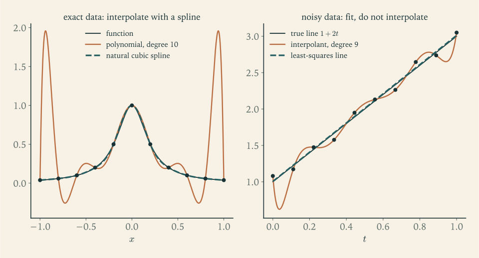
Figure 5.1 sets the two situations side by side. In the left panel the data are exact and the task is to fill in between them; the spline does this where the polynomial cannot. In the right panel the data are inexact and the task is to see through them; the fitted line does this where every interpolant fails.
A zero residual is therefore not a mark of a good model. The interpolant in Example 5.7 has residual zero and the fitted line has residual norm \(0.196\)
, and the line is the better description of the process that generated the data. How to quantify that judgment, how large a residual the noise explains, how uncertain the fitted coefficients are, and when an additional parameter is justified, are questions about random error, and they belong to Mathematical Statistics, where the linear model is studied as an inference problem (math.mathematical-statistics.linear-models-synthesis). The numerical analyst’s contribution is to compute the fit that statistics asks for without losing digits on the way.
The next chapter applies interpolation to a different end. If a function can be replaced by a polynomial that is close to it, the integral of the function can be replaced by the integral of the polynomial, which is elementary.
Exercises
-
Use Proposition 5.1 to find the number of equal subintervals that guarantees an error of at most \(10^{-4}\) when \(\sin x\) is replaced by its piecewise linear interpolant on \([0,\pi]\) .
Answer
\(\lVert f''\rVert_\infty=1\) , so \(h^2/8\le10^{-4}\) requires \(h\le0.0283\) and \(n\ge\pi/0.0283=111.1\) : use \(112\) subintervals.
-
Count coefficients and conditions to show that a cubic spline interpolant on \(n\) subintervals needs two extra conditions, and repeat the count for a quadratic spline, which is piecewise quadratic with \(s\) and \(s'\) continuous; say how many extra conditions it needs.
Answer
Cubic: \(4n\) coefficients; \(2n\) interpolation conditions and \(2(n-1)\) smoothness conditions leave \(4n-(4n-2)=2\) free. Quadratic: \(3n\) coefficients; \(2n\) interpolation conditions and \(n-1\) conditions for continuity of \(s'\) total \(3n-1\) , leaving one free, for example a slope at one end.
-
Compute the natural cubic spline through \((0,0)\) , \((1,1)\) , \((2,0)\) by solving for \(M_1\) , give the formula for \(s\) on \([0,1]\) , verify the slope at \(x=1\) from the left, and evaluate \(s(0.5)\) .
Solution
All spacings are \(h_i=1\) and the data slopes are \(\delta_0=1\) and \(\delta_1=-1\) . With \(M_0=M_2=0\) the single equation is
\[ M_0+4M_1+M_2=6(\delta_1-\delta_0)=-12, \]so \(M_1=-3\) . On \([0,1]\) the formula of Section 5.2 with \(x_0=0\) , \(x_1=1\) , \(y_0=0\) , \(y_1=1\) , \(M_0=0\) , \(M_1=-3\) gives
\[ s(x)=\frac{-3x^3}{6}+\Bigl(1+\frac{3}{6}\Bigr)x,\qquad\text{that is,}\qquad s(x)=-\tfrac12x^3+\tfrac32x . \]Check: \(s(0)=0\) , \(s(1)=1\) , \(s''(0)=0\) , \(s''(1)=-3=M_1\) . The slope from the left at the middle knot is \(s'(1)=-\tfrac32+\tfrac32=0\) . By the symmetry of the data about \(x=1\) , the piece on \([1,2]\) is the mirror image \(s(2-x)\) , whose slope at \(1\) is also \(0\) , so \(s'\) is continuous there, as it must be. Finally \(s(0.5)=0.6875\) , obtained from \(-\tfrac1{16}+\tfrac34\) . The spline rises to a smooth maximum at the middle knot; the parabola through the same points, \(2x-x^2\) , gives \(0.75\) at \(x=0.5\) .
-
Let \(s(x)=x^3\) on \([0,1]\) and \(s(x)=1+3(x-1)+3(x-1)^2+\alpha(x-1)^3\) on \([1,2]\) . Show that \(s\) is a cubic spline on \([0,2]\) for every \(\alpha\) , and find the value of \(\alpha\) for which it is a natural spline.
Answer
At \(x=1\) the left piece has \(s=1\) , \(s'=3\) , \(s''=6\) ; the right piece has \(s=1\) , \(s'=3\) , \(s''=2\cdot3=6\) . So \(s\) , \(s'\) , \(s''\) are continuous for every \(\alpha\) . The natural conditions are \(s''(0)=0\) , which holds since \(s''=6x\) on the left, and \(s''(2)=6+6\alpha=0\) , which requires \(\alpha=-1\) .
-
Let \(s\) be the clamped cubic spline interpolating \(f\) at the knots with \(s'(x_0)=f'(x_0)\) and \(s'(x_n)=f'(x_n)\) . Prove that \(\int(s'')^2\le\int(g'')^2\) for every twice continuously differentiable \(g\) that interpolates the same values and has the same two end slopes.
Solution
Put \(e=g-s\) . Since \(g\) and \(s\) interpolate the same values, \(e(x_i)=0\) at every knot; since they have the same end slopes, \(e'(x_0)=e'(x_n)=0\) . As in the proof of Theorem 5.5,
\[ \int_{x_0}^{x_n}(g'')^2\,dx=\int_{x_0}^{x_n}(s'')^2\,dx+\int_{x_0}^{x_n}(e'')^2\,dx+2\int_{x_0}^{x_n}s''e''\,dx , \]so it suffices to show that the last integral vanishes. On each subinterval \(s'''\) is a constant \(c_i\) , and integration by parts gives
\[ \int_{x_i}^{x_{i+1}}s''e''\,dx=\Bigl[s''e'\Bigr]_{x_i}^{x_{i+1}}-c_i\bigl(e(x_{i+1})-e(x_i)\bigr)=\Bigl[s''e'\Bigr]_{x_i}^{x_{i+1}} . \]Summing over \(i\) , the contributions at interior knots cancel in pairs because \(s''\) and \(e'\) are continuous, leaving \(s''(x_n)e'(x_n)-s''(x_0)e'(x_0)\) . In Theorem 5.5 this vanished because \(s''\) is zero at the ends; here it vanishes because \(e'\) is zero at the ends. Hence \(\int(g'')^2=\int(s'')^2+\int(e'')^2\ge\int(s'')^2\) . So the clamped spline minimizes the bending energy among interpolants with prescribed end slopes, just as the natural spline does among all interpolants.
-
From the clamped-spline errors in Example 5.3 compute the observed orders, predict the error for \(n=64\) , and explain why the ratio of successive errors approaches \(16\) .
Answer
The orders are \(\log_2(2.636\times10^{-5}/1.690\times10^{-6})=3.96\) , then \(3.98\) and \(3.99\) . The error behaves like \(Ch^4\) , so halving \(h\) divides it by \(2^4=16\) ; the prediction for \(n=64\) is \(6.716\times10^{-9}/16=4.2\times10^{-10}\) , and the computed value is \(4.21\times10^{-10}\) .
-
A student interpolates \(e^{x}\) on \([0,1]\) with a natural cubic spline, observes that the error decreases by a factor of only \(4\) when the number of knots is doubled, and concludes that the program has a bug. Explain why the observation is consistent with a correct program, where the error is concentrated, and what change restores fourth-order accuracy.
Answer
A factor of \(4\) per doubling is order \(2\) , which is exactly what the natural spline delivers when \(f''\) does not vanish at the ends: here \(f''(0)=1\) and \(f''(1)=e\) , and the end conditions force \(s''=0\) there. The error is concentrated in the first and last few subintervals and decays rapidly into the interior, where the spline is fourth-order accurate. Using the clamped spline with slopes \(1\) and \(e\) , or the not-a-knot spline, restores order four everywhere.
-
Fit a line \(y=x_1+x_2t\) to the data \((0,1)\) , \((1,2)\) , \((2,2)\) , \((3,4)\) by forming and solving the normal equations, list the residuals, and verify both orthogonality conditions.
Solution
The matrix \(A\) has columns \((1,1,1,1)\) and \((0,1,2,3)\) , and \(b=(1,2,2,4)\) . The entries of the normal equations are \(\sum1=4\) , \(\sum t_i=6\) , \(\sum t_i^2=14\) , \(\sum y_i=9\) , and \(\sum t_iy_i=0+2+4+12=18\) :
\[ \begin{pmatrix}4&6\\6&14\end{pmatrix}\begin{pmatrix}x_1\\x_2\end{pmatrix}=\begin{pmatrix}9\\18\end{pmatrix}. \]The determinant is \(56-36=20\) , and Cramer’s rule gives \(x_1=(9\cdot14-6\cdot18)/20=18/20\) and \(x_2=(4\cdot18-6\cdot9)/20=18/20\) . So \(x_1=0.9\) and \(x_2=0.9\) , and the fitted line is \(y=0.9+0.9t\) .
The fitted values are \(0.9\) , \(1.8\) , \(2.7\) , \(3.6\) , so the residuals \(y_i-(0.9+0.9t_i)\) are \(0.1\) , \(0.2\) , \(-0.7\) , \(0.4\) . They sum to \(0.1+0.2-0.7+0.4=0\) , which is orthogonality to the column of ones. Weighted by \(t_i\) they give \(0+0.2-1.4+1.2=0\) , which is orthogonality to the second column. Both conditions of Theorem 5.7 hold, so this line minimizes the sum of squared residuals, whose value is \(0.01+0.04+0.49+0.16=0.70\) .
-
Prove that when a least-squares line \(y=x_1+x_2t\) is fitted to data \((t_i,y_i)\) , the residuals sum to zero and the fitted line passes through the point \((\bar t,\bar y)\) of mean coordinates.
Solution
The matrix \(A\) has first column \((1,\dots,1)\) and second column \((t_1,\dots,t_m)\) . By Theorem 5.7 the residual \(r=b-Ax^\star\) of the least-squares solution satisfies \(A^{\top}r=0\) , and the first component of this vector equation is the inner product of \(r\) with the column of ones:
\[ \sum_{i=1}^{m}r_i=0 . \]That is the first claim. Now write out the residuals, \(r_i=y_i-x_1-x_2t_i\) , and sum: \(\sum_iy_i-mx_1-x_2\sum_it_i=0\) . Dividing by \(m\) gives \(\bar y=x_1+x_2\bar t\) , which says precisely that the point \((\bar t,\bar y)\) lies on the fitted line \(y=x_1+x_2t\) .
The argument uses only the presence of a constant column in \(A\) , so the same two facts hold for any linear least-squares model that includes a constant term: the residuals have mean zero, and the fitted function reproduces the mean of the observations at the mean of the regressors. A model without a constant term, such as \(y=x_2t\) , has neither property in general.
-
The model \(y=ce^{kt}\) is fitted to \((0,2.0)\) , \((1,3.3)\) , \((2,5.4)\) , \((3,9.0)\) by taking logarithms and fitting a line to \((t_i,\ln y_i)\) . Compute \(k\) and \(c\) , and explain why the result is not in general the minimizer of \(\sum_i(y_i-ce^{kt_i})^2\) .
Answer
With \(z_i=\ln y_i=(0.6931,1.1939,1.6864,2.1972)\) the least-squares line is \(z=0.6920+0.5005\,t\) , so \(k=0.5005\) and \(c=e^{0.6920}=1.998\) . The fitted values \(1.998\) , \(3.295\) , \(5.435\) , \(8.965\) are close to the data. The procedure minimizes \(\sum(\ln y_i-\ln c-kt_i)^2\) , which measures relative deviations and so weights small observations as heavily as large ones; minimizing \(\sum(y_i-ce^{kt_i})^2\) is a different, nonlinear problem with a slightly different solution.
-
Compute the QR factorization of the \(3\times2\) matrix with columns \((1,1,1)\) and \((1,2,3)\) by the Gram–Schmidt process, and use it to find the least-squares line for the data \((1,1)\) , \((2,2)\) , \((3,2)\) .
Solution
Let \(a_1=(1,1,1)\) and \(a_2=(1,2,3)\) . Gram–Schmidt: \(r_{11}=\lVert a_1\rVert_2=\sqrt3\) and \(q_1=(1,1,1)/\sqrt3\) . Then \(r_{12}=q_1^{\top}a_2=6/\sqrt3=2\sqrt3\) and \(v_2=a_2-r_{12}q_1=(1,2,3)-(2,2,2)=(-1,0,1)\) , so \(r_{22}=\sqrt2\) and \(q_2=(-1,0,1)/\sqrt2\) . Thus
\[ Q=\begin{pmatrix}1/\sqrt3&-1/\sqrt2\\1/\sqrt3&0\\1/\sqrt3&1/\sqrt2\end{pmatrix},\qquad R=\begin{pmatrix}\sqrt3&2\sqrt3\\0&\sqrt2\end{pmatrix}. \]For the data, \(t=(1,2,3)\) is the second column and \(b=(1,2,2)\) . Then \(Q^{\top}b=\bigl(5/\sqrt3,\ 1/\sqrt2\bigr)\) , and back substitution in \(Rx=Q^{\top}b\) gives \(x_2=\tfrac12\) from \(\sqrt2\,x_2=1/\sqrt2\) , and then \(\sqrt3\,x_1+2\sqrt3\cdot\tfrac12=5/\sqrt3\) , so \(x_1=\tfrac23\) . The least-squares line is \(y=\tfrac23+\tfrac12t\) . Its residuals are \(-\tfrac16,\tfrac13,-\tfrac16\) , which sum to zero and are orthogonal to \((1,2,3)\) .
-
For a matrix \(A\) with independent columns let \(\sigma_{\max}^2\) and \(\sigma_{\min}^2\) denote the largest and smallest eigenvalues of \(A^{\top}A\) . Show that \(\sigma_{\max}\) and \(\sigma_{\min}\) are the maximum and minimum of \(\lVert Az\rVert_2/\lVert z\rVert_2\) over \(z\ne0\) , and deduce that \(\kappa_2(A^{\top}A)=\kappa_2(A)^2\) .
Solution
The matrix \(B=A^{\top}A\) is symmetric, and positive definite because the columns of \(A\) are independent. By the spectral theorem for symmetric matrices it has an orthonormal basis of eigenvectors \(v_1,\dots,v_n\) with positive eigenvalues \(\lambda_1\ge\dots\ge\lambda_n\) . For \(z=\sum_jc_jv_j\ne0\) ,
\[ \frac{\lVert Az\rVert_2^2}{\lVert z\rVert_2^2}=\frac{z^{\top}Bz}{z^{\top}z}=\frac{\sum_j\lambda_jc_j^2}{\sum_jc_j^2}, \]a weighted average of the eigenvalues. It lies between \(\lambda_n\) and \(\lambda_1\) and attains those values at \(z=v_n\) and \(z=v_1\) . Taking square roots, the maximum and minimum of \(\lVert Az\rVert_2/\lVert z\rVert_2\) are \(\sigma_{\max}=\sqrt{\lambda_1}\) and \(\sigma_{\min}=\sqrt{\lambda_n}\) , so \(\kappa_2(A)=\sqrt{\lambda_1/\lambda_n}\) .
Apply the same reasoning to \(B\) itself. \(B^{\top}B=B^2\) has the same eigenvectors with eigenvalues \(\lambda_j^2\) , so the stretching factors of \(B\) range between \(\lambda_n\) and \(\lambda_1\) , and \(\kappa_2(B)=\lambda_1/\lambda_n\) . Therefore \(\kappa_2(A^{\top}A)=\lambda_1/\lambda_n=\kappa_2(A)^2\) .
-
A least-squares problem with a small residual has \(\kappa_2(A)=10^{5}\) and is solved in double precision. Using the rule of thumb of Chapter 1, estimate the number of correct digits obtained from the normal equations and from QR, and find the largest \(\kappa_2(A)\) for which the normal equations can be expected to give any correct digits.
Answer
Normal equations: relative error about \(\kappa^2u=10^{10}\times1.1\times10^{-16}\approx10^{-6}\) , six correct digits. QR, the residual being small: about \(\kappa u\approx10^{-11}\) , eleven digits. The normal equations give no correct digits once \(\kappa^2u\ge1\) , that is, for \(\kappa_2(A)\) above \(u^{-1/2}\approx9.5\times10^{7}\) .
-
Let \(A\) have rows \((1,1)\) , \((\epsilon,0)\) , \((0,\epsilon)\) with \(\epsilon=10^{-8}\) . Compute \(A^{\top}A\) exactly and as it is stored in double precision, show that the stored matrix is singular although \(A\) has independent columns, and compute \(\kappa_2(A)\) .
Solution
The columns of \(A\) are \((1,\epsilon,0)\) and \((1,0,\epsilon)\) , so
\[ A^{\top}A=\begin{pmatrix}1+\epsilon^2&1\\1&1+\epsilon^2\end{pmatrix}, \]with determinant \((1+\epsilon^2)^2-1=2\epsilon^2+\epsilon^4>0\) . Exactly, the matrix is nonsingular, in agreement with Theorem 5.7, since the two columns of \(A\) are independent.
In double precision \(\epsilon^2=10^{-16}\) , which is smaller than the unit roundoff \(u=1.11\times10^{-16}\) , so \(1+\epsilon^2\) rounds to \(1\) . Hence the stored matrix has all four entries equal to \(1\) ; its determinant is \(0\) and it is singular. The information that distinguished the two columns of \(A\) , carried by the entries \(\epsilon\) , has been squared out of existence.
The eigenvalues of the exact \(A^{\top}A\) are \(\epsilon^2\) , for the eigenvector \((1,-1)\) , and \(2+\epsilon^2\) , for \((1,1)\) . By Exercise 5.12,
\[ \kappa_2(A)=\sqrt{2+\epsilon^2}/\epsilon\approx1.4\times10^{8} . \]This exceeds \(u^{-1/2}\) , the threshold of Exercise 5.13. The problem itself is solvable to about eight digits, since \(\kappa_2(A)u\approx10^{-8}\) , and a QR-based solver achieves that; for instance with \(b=(2,\epsilon,\epsilon)\) it returns the exact solution \((1,1)\) to eight digits. The normal equations cannot even be set up.
-
For the five points \(t=-2,-1,0,1,2\) show that the columns built from \(1\) , \(t\) , and \(t^2-2\) are mutually orthogonal, so that \(A^{\top}A\) is diagonal, and use this to fit a quadratic to the values \(y=(0,1,1,3,7)\) without solving a system.
Answer
\(\sum t_i=0\) , \(\sum(t_i^2-2)=10-10=0\) , and \(\sum t_i(t_i^2-2)=0\) by oddness, so the three columns are orthogonal, with squared norms \(5\) , \(10\) , and \(14\) . Each coefficient is then an inner product divided by a squared norm: \(c_0=\sum y_i/5=12/5\) , \(c_1=\sum t_iy_i/10=16/10\) , \(c_2=\sum(t_i^2-2)y_i/14=8/14\) . The fit is \(y=2.4+1.6\,t+\tfrac47(t^2-2)\) .
-
A colleague argues: “The degree-\(9\) polynomial through my ten measurements has zero residual, the fitted line has a residual of \(0.2\) , so the polynomial is the better model.” Explain what is wrong with the argument, referring to Example 5.7 and Theorem 4.8.
Hint
The residual measures how well a model reproduces the observations, errors included, not how well it describes what produced them. Count parameters: ten coefficients fitted to ten numbers must give zero residual whatever the data are. Then use Theorem 4.8(a) with \(\Lambda_9\approx18\) to bound what the errors in the data can do to the interpolant between the nodes, and compare with Example 5.7.
-
For the natural spline of Exercise 5.3, compute \(\int_0^2s''(x)^2\,dx\) , compare it with the same integral for the parabola through the three points, and say which theorem predicts the outcome.
Solution
From Exercise 5.3, \(s(x)=-\tfrac12x^3+\tfrac32x\) on \([0,1]\) , so \(s''(x)=-3x\) there, and by symmetry \(s''(x)=-3(2-x)\) on \([1,2]\) . Then
\[ \int_0^1(-3x)^2\,dx=\int_0^19x^2\,dx=3, \]the second subinterval contributes the same amount, and the total is \(6\) .
The parabola through \((0,0)\) , \((1,1)\) , \((2,0)\) is \(g(x)=2x-x^2\) , with \(g''\equiv-2\) , so
\[ \int_0^2(-2)^2\,dx=8 . \]The spline bends less in the mean-square sense: \(6<8\) . Theorem 5.5 predicts exactly this, since the parabola is a twice continuously differentiable interpolant of the same data and is not the natural spline. The spline achieves its smaller energy by having zero curvature at the two ends and concentrating the bending near the middle knot, where \(s''=-3\) ; the parabola bends uniformly. The proof of the theorem even gives the difference: \(8-6=2=\int_0^2(g''-s'')^2\,dx\) .
-
Estimate the number of arithmetic operations needed to construct and evaluate once a natural cubic spline through \(1001\) points, given that a tridiagonal system of size \(n\) is solved in about \(8n\) operations, and compare with the \(n^2/2\) divisions of a divided-difference table.
Answer
There are \(999\) unknown moments, so the solve costs about \(8\times10^{3}\) operations, plus a comparable number to form the right-hand side and about ten operations for one evaluation: roughly \(10^{4}\) in all. A divided-difference table for \(1001\) points needs about \(n^2/2=5\times10^{5}\) divisions before any evaluation, and the resulting polynomial would be useless on equally spaced data in any case.
-
Use Lemma 5.3 to show that the matrix with rows \((4,1,0)\) , \((1,4,1)\) , \((0,1,4)\) is nonsingular, and give a \(2\times2\) matrix in which each diagonal entry equals the sum of the other magnitudes in its row and which is singular.
Answer
Row by row, \(4>1\) , \(4>1+1\) , and \(4>1\) , so the matrix is strictly diagonally dominant and nonsingular by Lemma 5.3. The matrix with rows \((1,1)\) and \((1,1)\) has each diagonal entry equal to the off-diagonal magnitude in its row and is singular, so strictness cannot be dropped from the lemma.
-
On a uniform grid with spacing \(h\) , a piecewise cubic Hermite interpolant uses the exact values of \(f\) and \(f'\) at every knot. Use the error formula of Section 4.6 to show that its error is at most \(h^4\lVert f''''\rVert_\infty/384\) , compare this with the clamped-spline bound, and state what each method requires and what smoothness each delivers.
Hint
On \([x_i,x_{i+1}]\) the factor \((x-x_i)^2(x-x_{i+1})^2\) is the square of the quantity maximized in Exercise 4.8, so it is at most \((h^2/4)^2\) ; divide by \(24\) . The spline constant is five times larger. Then compare the inputs, values and slopes at every knot against values alone plus two end conditions, and the outputs, one continuous derivative against two.