Solve the system

by elimination in double precision, exactly as taught in a first course: subtract \(10^{20}\) times the first equation from the second and back-substitute. The computer returns \(x=(0,1)\) . The true solution is \((1,1)\) to twenty digits. The matrix is not close to singular; its determinant is \(-1\) to twenty digits. Swap the two equations and repeat the same procedure, and the answer is \((1,1)\) .

Now a different experiment. The \(12\times12\) Hilbert matrix, with entries \(1/(i+j-1)\) , is nonsingular, and a careful library routine solves a system with it and returns a vector \(\hat x\) that satisfies the equations to sixteen digits: the residual \(b-A\hat x\) is at the level of rounding. Yet \(\hat x\) has at most one correct digit.

The two failures have opposite causes, and separating them is the purpose of this chapter. The first is an unstable algorithm applied to a harmless problem, and it is cured by pivoting. The second is a stable algorithm applied to an ill-conditioned problem, and it cannot be cured, only diagnosed. The diagnosis needs a way to measure the sensitivity of a linear system, which is the condition number of a matrix, and a clear understanding of what the residual does and does not say about the error. These are the ideas of Chapter 1, backward error and conditioning, in the setting where they matter most: nearly every method in the rest of the book ends by solving a linear system.

7.1 Elimination as a factorization

Gaussian elimination, as developed in Linear Algebra (math.linear-algebra.elimination-as-structured-reduction), reduces \(Ax=b\) to an upper triangular system by subtracting multiples of each pivot row from the rows below it. At step \(k\) the multipliers are \(m_{ik}=a^{(k)}_{ik}/a^{(k)}_{kk}\) for \(i>k\) , where \(a^{(k)}\) denotes the entries after \(k-1\) steps, and row \(i\) is replaced by row \(i\) minus \(m_{ik}\) times row \(k\) . The numerical analyst’s view of the process is that it computes a factorization.

Once \(A=LU\) is known, \(Ax=b\) is solved in two triangular stages: forward substitution for \(Ly=b\) , then back substitution for \(Ux=y\) . The work is unevenly divided. Step \(k\) of the factorization performs about \((n-k)^2\) multiplications, so the total is about \(\tfrac13n^3\) multiplications and as many subtractions; each triangular solve costs about \(\tfrac12n^2\) . For \(n=1000\) the factorization costs a few hundred million operations and each additional right-hand side a million. This is the reason never to compute \(A^{-1}\) in order to solve a system: the inverse costs three times as much as the factorization, and the factors do everything the inverse could do, more accurately.

7.2 Why pivoting, and what it guarantees

Theorem 7.1 can fail for a perfectly good matrix: if \(a_{11}=0\) the first step is impossible although \(A\) may be nonsingular. The remedy is to interchange rows. What the opening example shows is that in floating-point arithmetic a pivot that is merely small is as dangerous as one that is zero.

7.3 Measuring sensitivity: norms and the condition number

To speak of small perturbations of vectors and matrices we need to measure their size.

By definition \(\lVert Ax\rVert\le\lVert A\rVert\lVert x\rVert\) for every \(x\) , and consequently \(\lVert AB\rVert\le\lVert A\rVert\lVert B\rVert\) . The induced norms can be computed:

the largest absolute row sum, the largest absolute column sum, and the square root of the largest eigenvalue of \(A^{\top}A\) . For the first: \(\lvert(Ax)_i\rvert\le\sum_j\lvert a_{ij}\rvert\lvert x_j\rvert\le\lVert x\rVert_\infty\sum_j\lvert a_{ij}\rvert\) , so \(\lVert Ax\rVert_\infty\) is at most \(\lVert x\rVert_\infty\) times the largest row sum; and equality is attained by the vector with \(x_j=\operatorname{sign}a_{ij}\) for a row \(i\) of largest sum. The second is Exercise 7.7, and the third was the content of Exercise 5.12.

Since \(1=\lVert I\rVert=\lVert AA^{-1}\rVert\le\lVert A\rVert\lVert A^{-1}\rVert\) , always \(\kappa(A)\ge1\) . The number depends on the norm, but only by modest factors, and the subscript on \(\kappa\) records which norm is meant.

Both bounds are attained for suitable perturbations, so \(\kappa(A)\) is exactly the factor by which relative errors in the data can be magnified in the solution: it is the condition number, in the sense of Chapter 1, of the problem of solving \(Ax=b\) . Combine part (b) with backward stability. A stable solver returns the exact solution of a system with \(\lVert\delta A\rVert/\lVert A\rVert\) of order \(u\) , so its relative error is of order \(\kappa(A)\,u\) . The rule of thumb: solving a linear system in double precision loses about \(\log_{10}\kappa(A)\) of the sixteen digits.

One more characterization, which we state without proof, makes the number vivid. In the \(2\) -norm, \(1/\kappa_2(A)\) is the relative distance from \(A\) to the nearest singular matrix: the smallest \(\lVert\delta A\rVert_2/\lVert A\rVert_2\) for which \(A+\delta A\) is singular. An ill-conditioned matrix is one that is nearly singular, in a precise and scale-free sense. The determinant is useless for this purpose. The matrix \(0.1\,I\) of order \(100\) has determinant \(10^{-100}\) and condition number \(1\) .

7.4 What a small residual does and does not certify

The error \(\hat x-x\) of a computed solution is unknown. The residual \(r=b-A\hat x\) can be computed. Theorem 7.6(a), read with \(\delta b=-r\) , relates the two, and running the same argument with the roles of \(A\) and \(A^{-1}\) exchanged gives a lower bound as well:

When \(\kappa(A)\) is near \(1\) the relative residual and the relative error are nearly the same thing. When \(\kappa(A)\) is large they can differ by that factor in either direction. And there is an asymmetry that catches everyone once. A backward stable solver produces a small residual whatever the conditioning: from \((A+\delta A)\hat x=b\) we have \(r=\delta A\,\hat x\) , so \(\lVert r\rVert\le\lVert\delta A\rVert\lVert\hat x\rVert\) , which is of order \(u\lVert A\rVert\lVert\hat x\rVert\) . A small residual therefore certifies that the algorithm was stable. It says nothing about the accuracy of \(\hat x\) unless the condition number is known.

Example 7.5: Hilbert matrices

The Hilbert matrix \(H_n\) has entries \(1/(i+j-1)\) . Solve \(H_nx=b\) in double precision by elimination with partial pivoting, with \(b\) chosen so that the solution is the vector of ones.

\(n\)	\(\kappa_2(H_n)\)	\(\kappa_2(H_n)\,u\)	relative error of \(\hat x\)	relative residual
\(4\)	\(1.55\times10^{4}\)	\(1.7\times10^{-12}\)	\(2\times10^{-13}\)	below \(10^{-15}\)
\(6\)	\(1.50\times10^{7}\)	\(1.7\times10^{-9}\)	\(5\times10^{-10}\)	below \(10^{-15}\)
\(8\)	\(1.53\times10^{10}\)	\(1.7\times10^{-6}\)	\(3\times10^{-7}\)	below \(10^{-15}\)
\(10\)	\(1.60\times10^{13}\)	\(1.8\times10^{-3}\)	\(6\times10^{-4}\)	below \(10^{-15}\)
\(12\)	\(1.7\times10^{16}\)	\(1.9\)	between \(10^{-2}\) and \(1\)	below \(10^{-15}\)

The error column is rounding noise, printed to one digit as obtained on the machine used for this book; on another machine or with another library only its orders of magnitude will recur. The pattern is unmistakable. The condition number grows by a factor of about \(30\) with each unit increase in \(n\) . The error follows \(\kappa_2(H_n)u\) , staying somewhat below it. The residual never rises above the level of rounding. At \(n=12\) the solver has done its job perfectly, the equations are satisfied to sixteen digits, and the answer has at most one correct digit.

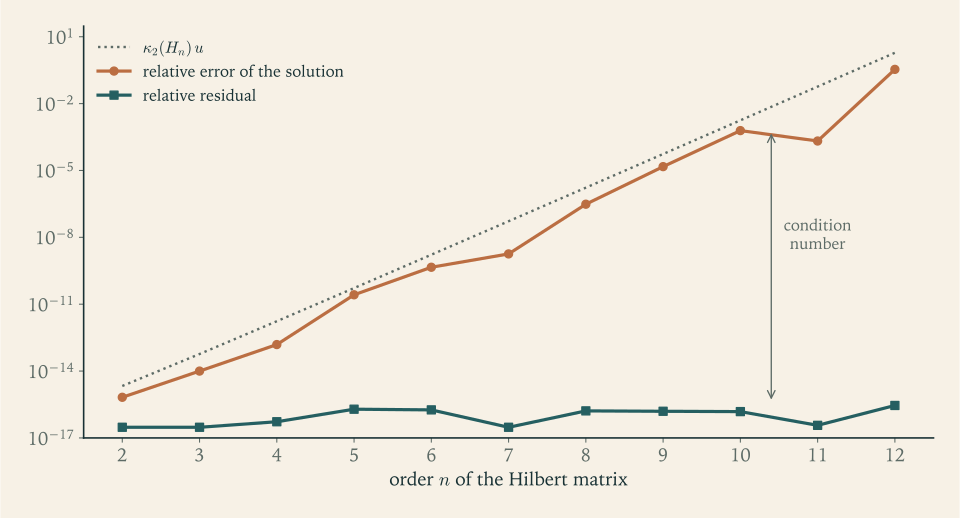
Figure 7.1 is the picture to recall whenever a computed solution “checks” when substituted back. The lower curve is what the check sees. The upper curve is what the user cares about. The vertical distance between them is the condition number.

Common mistake. Verifying a computed solution by substituting it into the equations and concluding from a small residual that it is accurate. The check tests backward stability, which good software has anyway. To assess accuracy, estimate the condition number, which library solvers report or warn about, and multiply it by the relative uncertainty of the data and by \(u\) . If \(\kappa(A)u\) is not small, no solver can help; the remedy is to reformulate the problem, for example by choosing a better basis as in Section 5.5, or to obtain more accurate data.

One device does extract more accuracy when the data are exact and the conditioning is moderate. In iterative refinement the residual \(r=b-A\hat x\) is computed, in higher precision if possible, the correction equation \(Ad=r\) is solved with the factors already in hand at a cost of order \(n^2\) , and \(\hat x\) is replaced by \(\hat x+d\) . Each pass reduces the error by a factor of about \(\kappa(A)u\) .

7.5 Structure: symmetric positive definite and banded systems

Matrices from applications are seldom arbitrary. Two kinds of structure occur constantly, and each makes elimination cheaper and safer.

A symmetric matrix \(A\) is positive definite if \(x^{\top}Ax>0\) for every \(x\ne0\) . The matrix \(A^{\top}A\) of the normal equations is of this kind, and so are the matrices arising from boundary-value problems in Chapter 10.

The factor is computed column by column from the equations \(a_{ij}=\sum_{k\le j}l_{ik}l_{jk}\) : \(l_{jj}=\bigl(a_{jj}-\sum_{k<j}l_{jk}^2\bigr)^{1/2}\) and \(l_{ij}=\bigl(a_{ij}-\sum_{k<j}l_{ik}l_{jk}\bigr)/l_{jj}\) for \(i>j\) . The cost is about \(\tfrac16n^3\) multiplications, half that of an LU factorization, and no pivoting is needed: the identity \(a_{ii}=\sum_kl_{ik}^2\) shows that no entry of \(L\) can exceed \(\sqrt{a_{ii}}\) , so there is no growth. Cholesky factorization is backward stable unconditionally. It is also the standard test of positive definiteness: the algorithm succeeds if and only if every quantity under a square root is positive.

Exercises

1. Compute the LU factorization of the matrix with rows \((1,2,1)\) , \((2,6,3)\) , \((3,10,8)\) without pivoting, use it to solve \(Ax=b\) for \(b=(4,11,21)\) , and give \(\det A\) .

   Solution

   Factorization. The first pivot is \(1\) , with multipliers \(m_{21}=2\) and \(m_{31}=3\) . Subtracting, row 2 becomes \((0,2,1)\) and row 3 becomes \((0,4,5)\) . The second pivot is \(2\) , with multiplier \(m_{32}=2\) , and row 3 becomes \((0,0,3)\) . Hence

   \[ L=\begin{pmatrix}1&0&0\\2&1&0\\3&2&1\end{pmatrix},\qquad U=\begin{pmatrix}1&2&1\\0&2&1\\0&0&3\end{pmatrix}. \]

   Multiplying out: the third row of \(LU\) is \(3(1,2,1)+2(0,2,1)+(0,0,3)=(3,10,8)\) , as required, and the second is \(2(1,2,1)+(0,2,1)=(2,6,3)\) .

   Solve. Forward substitution in \(Ly=b\) with \(b=(4,11,21)\) : \(y_1=4\) , \(y_2=11-8=3\) , \(y_3=21-12-6=3\) , so \(y=(4,3,3)\) . Back substitution in \(Ux=y\) : \(x_3=1\) ; \(2x_2+1=3\) gives \(x_2=1\) ; \(x_1+2+1=4\) gives \(x_1=1\) . So \(x=(1,1,1)\) .

   Determinant. Since \(\det L=1\) , \(\det A=\det U\) , the product of the pivots: \(\det A=1\cdot2\cdot3=6\) . No interchanges were needed, so no sign change enters.

2. Show that the elimination phase for an \(n\times n\) system needs about \(\tfrac13n^3\) multiplications and each triangular solve about \(\tfrac12n^2\) , and estimate the cost of solving one system with ten different right-hand sides for \(n=1000\) , with and without reuse of the factorization.

   Answer

   Step \(k\) computes \(n-k\) multipliers and updates an \((n-k)\times(n-k)\) block, so the multiplications number \(\sum_{k=1}^{n-1}(n-k)^2\approx\tfrac13n^3\) . A triangular solve uses \(1+2+\dots+(n-1)\approx\tfrac12n^2\) . For \(n=1000\) : one factorization costs about \(3.3\times10^{8}\) and each right-hand side \(10^{6}\) , so ten right-hand sides cost \(3.4\times10^{8}\) with reuse and \(3.3\times10^{9}\) if the elimination is repeated each time.

3. Prove that the matrix with rows \((0,1)\) and \((1,1)\) has no factorization \(A=LU\) with \(L\) unit lower triangular and \(U\) upper triangular, and give a permutation \(P\) and factors with \(PA=LU\) .

   Solution

   Suppose \(A=LU\) with \(L=\begin{pmatrix}1&0\\l&1\end{pmatrix}\) and \(U=\begin{pmatrix}u_{11}&u_{12}\\0&u_{22}\end{pmatrix}\) . The \((1,1)\) entry of the product is \(u_{11}\) , which must equal \(a_{11}=0\) . The \((2,1)\) entry of the product is \(l\,u_{11}=0\) , which must equal \(a_{21}=1\) . These are contradictory, so no such factorization exists. The same contradiction arises whenever \(a_{11}=0\) and the first column is not zero, in agreement with Theorem 7.1, whose hypothesis here is that the \(1\times1\) leading submatrix \((0)\) be nonsingular.

   Interchanging the rows gives

   \[ PA=\begin{pmatrix}0&1\\1&0\end{pmatrix}\begin{pmatrix}0&1\\1&1\end{pmatrix}=\begin{pmatrix}1&1\\0&1\end{pmatrix}, \]

   which is already upper triangular, so \(PA=LU\) with \(L=I\) and \(U=\begin{pmatrix}1&1\\0&1\end{pmatrix}\) . The matrix \(A\) is nonsingular, with determinant \(-1\) ; it merely needed its rows in a different order, as Theorem 7.2 guarantees is always possible.

4. In decimal arithmetic with three significant digits, solve the system \(10^{-4}x_1+x_2=1\) , \(x_1+x_2=2\) by elimination without interchange and then with the rows interchanged, rounding after every operation, and compare with the exact solution to four digits.

   Solution

   Without interchange. The pivot is \(10^{-4}\) and the multiplier is \(10^{4}\) . The new \((2,2)\) entry is \(1-10^{4}=-9999\) , which rounds to \(-1.00\times10^{4}\) ; the new right-hand side is \(2-10^{4}=-9998\) , which also rounds to \(-1.00\times10^{4}\) . Then \(\hat x_2=1.00\) and \(\hat x_1=(1-1.00)/10^{-4}=0\) . The computed solution is \(\hat x=(0,1)\) .

   With interchange. The system is \(x_1+x_2=2\) , \(10^{-4}x_1+x_2=1\) . The multiplier is \(10^{-4}\) . The new \((2,2)\) entry is \(1-10^{-4}=0.9999\) , which rounds to \(1.00\) ; the new right-hand side is \(1-2\times10^{-4}=0.9998\) , which rounds to \(1.00\) . Then \(\hat x_2=1.00\) and \(\hat x_1=2-1.00=1.00\) . The computed solution is \(\hat x=(1,1)\) .

   Exact. Subtracting the equations, \((1-10^{-4})x_1=1\) , so \(x_1=1.0001\ldots\) and \(x_2=0.9999\ldots\) ; to four digits the solution is \((1.000,\,0.9999)\) . The pivoted computation is correct to the three digits carried. The unpivoted one has \(x_1\) entirely wrong. In it the multiplier \(10^{4}\) scaled the first equation so that the entries \(1\) and \(2\) of the second equation fell below the third digit and were rounded away; the second equation was effectively replaced by a multiple of the first. This is Example 7.2 in miniature, with the threshold set by three digits instead of sixteen.

5. Prove that elimination with partial pivoting has growth factor \(\rho\le2^{n-1}\) .

   Solution

   Let \(M_k=\max_{i,j}\lvert a^{(k)}_{ij}\rvert\) be the largest magnitude among the entries of the matrix at the start of step \(k\) , so \(M_1=\max\lvert a_{ij}\rvert\) . Row interchanges permute entries and do not change \(M_k\) . After the interchange, step \(k\) leaves rows \(1,\dots,k\) unchanged and replaces each entry in a later row by

   \[ a^{(k+1)}_{ij}=a^{(k)}_{ij}-m_{ik}\,a^{(k)}_{kj},\qquad i>k . \]

   With partial pivoting \(\lvert m_{ik}\rvert\le1\) , so by the triangle inequality

   \[ \lvert a^{(k+1)}_{ij}\rvert\le\lvert a^{(k)}_{ij}\rvert+\lvert a^{(k)}_{kj}\rvert\le2M_k . \]

   Hence \(M_{k+1}\le2M_k\) . There are \(n-1\) elimination steps, so \(M_k\le2^{k-1}M_1\le2^{n-1}M_1\) for every stage \(k\le n\) , and dividing by \(M_1\) gives \(\rho\le2^{n-1}\) . Example 7.3 shows that the bound is attained: there every multiplier has magnitude exactly \(1\) and the entries of the last column add with the same sign at every step.

6. For the matrix \(A\) with rows \((1,-2)\) and \((3,4)\) , compute \(\lVert A\rVert_1\) , \(\lVert A\rVert_\infty\) , and \(\lVert A\rVert_2\) , find \(A^{-1}\) , and compute \(\kappa_\infty(A)\) and \(\kappa_1(A)\) .

   Answer

   Column sums \(4\) and \(6\) give \(\lVert A\rVert_1=6\) ; row sums \(3\) and \(7\) give \(\lVert A\rVert_\infty=7\) . \(A^{\top}A\) has rows \((10,10)\) and \((10,20)\) , with eigenvalues \(15\pm5\sqrt5\) , so \(\lVert A\rVert_2=\sqrt{26.18}=5.117\) . The inverse is \(\tfrac1{10}\) times the matrix with rows \((4,2)\) and \((-3,1)\) , with \(\lVert A^{-1}\rVert_\infty=0.6\) and \(\lVert A^{-1}\rVert_1=0.7\) . Hence \(\kappa_\infty(A)=7\times0.6=4.2\) and \(\kappa_1(A)=6\times0.7=4.2\) .

7. Prove that the matrix norm induced by the vector \(1\) -norm is the largest absolute column sum.

   Solution

   Let \(c_j=\sum_i\lvert a_{ij}\rvert\) be the absolute sum of column \(j\) and \(c=\max_jc_j\) . For any \(x\) ,

   \[ \lVert Ax\rVert_1=\sum_i\Bigl\lvert\sum_ja_{ij}x_j\Bigr\rvert\le\sum_i\sum_j\lvert a_{ij}\rvert\lvert x_j\rvert=\sum_j\lvert x_j\rvert\,c_j\le c\sum_j\lvert x_j\rvert=c\,\lVert x\rVert_1 , \]

   where the order of summation was exchanged in the middle step. So \(\lVert Ax\rVert_1/\lVert x\rVert_1\le c\) for every \(x\ne0\) , and the induced norm is at most \(c\) .

   For the reverse inequality choose a column \(j^\star\) with \(c_{j^\star}=c\) and take \(x=e_{j^\star}\) , the unit vector with a \(1\) in position \(j^\star\) . Then \(\lVert x\rVert_1=1\) and \(Ax\) is column \(j^\star\) of \(A\) , so \(\lVert Ax\rVert_1=c\) . The maximum of the ratio is therefore exactly \(c\) : the induced \(1\) -norm is the largest absolute column sum. The \(\infty\) -norm case in Section 7.3 is the same argument with rows and columns exchanged, the maximizing vector there being a vector of signs.

8. Show that \(\kappa(\alpha A)=\kappa(A)\) for every nonzero scalar \(\alpha\) and that \(\kappa(AB)\le\kappa(A)\kappa(B)\) , and explain what the first property implies about using the size of the entries, or of the determinant, to judge conditioning.

   Answer

   \((\alpha A)^{-1}=\alpha^{-1}A^{-1}\) , so \(\kappa(\alpha A)=\lvert\alpha\rvert\lVert A\rVert\cdot\lvert\alpha\rvert^{-1}\lVert A^{-1}\rVert=\kappa(A)\) . And \(\kappa(AB)=\lVert AB\rVert\lVert B^{-1}A^{-1}\rVert\le\lVert A\rVert\lVert B\rVert\lVert B^{-1}\rVert\lVert A^{-1}\rVert\) . Scaling a matrix changes its entries and multiplies its determinant by \(\alpha^{n}\) without changing its conditioning, so neither small entries nor a small determinant indicates ill-conditioning.

9. Let \(A\) have rows \((1.01,0.99)\) and \((0.99,1.01)\) and let \(b=(2,2)\) , so that \(x=(1,1)\) . For the candidates \(\hat x=(2,0)\) and \(\tilde x=(1.01,1.01)\) compute the residuals and the errors in the \(\infty\) -norm, compute \(\kappa_\infty(A)\) , and check both against Corollary 7.7.

   Solution

   The exact solution is \(x=(1,1)\) , since each row sums to \(2\) . The determinant is \(1.01^2-0.99^2=0.04\) , so

   \[ A^{-1}=\frac{1}{0.04}\begin{pmatrix}1.01&-0.99\\-0.99&1.01\end{pmatrix}=\begin{pmatrix}25.25&-24.75\\-24.75&25.25\end{pmatrix}, \]

   with \(\lVert A^{-1}\rVert_\infty=50\) and \(\lVert A\rVert_\infty=2\) . Hence \(\kappa_\infty(A)=2\times50=100\) .

   First candidate. \(A\hat x=(2.02,1.98)\) , so the residual is \((-0.02,\,0.02)\) , of relative size \(0.02/2=0.01\) . The error is \(\hat x-x=(1,-1)\) , of relative size \(1\) .

   Second candidate. \(A\tilde x=(2.02,2.02)\) , so the residual is \((-0.02,\,-0.02)\) , again of relative size \(0.01\) . The error is \((0.01,0.01)\) , of relative size \(0.01\) .

   Corollary 7.7 allows any relative error between \(0.01/100=10^{-4}\) and \(100\times0.01=1\) for a relative residual of \(0.01\) , and both candidates comply. The first attains the upper bound exactly: its error \((1,-1)\) lies along the direction that \(A\) shrinks most, by the factor \(0.02\) . The second has error along \((1,1)\) , which \(A\) stretches by \(2\) , and for it the residual and the error are of equal relative size. Two candidates with identical residual norms differ by a factor of \(100\) in accuracy, and the residual alone cannot tell them apart.

10. Give a matrix with determinant \(10^{-100}\) and condition number \(1\) , and a matrix with determinant \(1\) and condition number larger than \(10^{8}\) , and state what the examples show.

    Answer

    \(0.1\,I\) of order \(100\) has determinant \(10^{-100}\) and condition number \(1\) . The diagonal matrix with entries \(10^{5}\) and \(10^{-5}\) has determinant \(1\) and condition number \(10^{10}\) . The determinant measures volume scaling, which depends on the units; the condition number measures the ratio of largest to smallest stretching, which is what governs sensitivity.

11. A user solves a \(12\times12\) Hilbert system in double precision, substitutes the result into the equations, finds agreement to sixteen digits, and reports the solution as accurate. Explain the error in the reasoning and estimate from Example 7.5 how many digits of the solution can be trusted.

    Answer

    The substitution computes the residual, and a backward stable solver makes the residual small for every nonsingular matrix. By Corollary 7.7 the relative error can exceed the relative residual by the factor \(\kappa_2(H_{12})=1.7\times10^{16}\) . Example 7.5 shows that the actual relative error is between \(10^{-2}\) and \(1\) : at most one digit of the solution can be trusted.

12. Compute the Cholesky factor of the matrix with rows \((9,3,3)\) , \((3,5,1)\) , \((3,1,5)\) and use it to solve \(Ax=b\) for \(b=(15,9,9)\) .

    Solution

    Column by column: \(l_{11}=\sqrt9=3\) , \(l_{21}=3/3=1\) , \(l_{31}=3/3=1\) ; then \(l_{22}=\sqrt{5-1^2}=2\) and \(l_{32}=(1-1\cdot1)/2=0\) ; finally \(l_{33}=\sqrt{5-1^2-0^2}=2\) . So

    \[ L=\begin{pmatrix}3&0&0\\1&2&0\\1&0&2\end{pmatrix}, \]

    and one checks \(LL^{\top}=A\) : for example the \((2,2)\) entry is \(1+4=5\) and the \((3,2)\) entry is \(1\cdot1+0\cdot2=1\) . Every quantity under a square root was positive, so \(A\) is positive definite.

    To solve \(Ax=b\) with \(b=(15,9,9)\) , first \(Ly=b\) : \(y_1=15/3=5\) , \(y_2=(9-5)/2=2\) , \(y_3=(9-5-0)/2=2\) , so \(y=(5,2,2)\) . Then \(L^{\top}x=y\) , an upper triangular system with rows \((3,1,1)\) , \((0,2,0)\) , \((0,0,2)\) : \(x_3=1\) , \(x_2=1\) , and \(3x_1+1+1=5\) gives \(x_1=1\) . So \(x=(1,1,1)\) , and indeed each row of \(A\) sums to the corresponding entry of \(b\) .

13. Attempt the Cholesky factorization of the symmetric matrix with rows \((1,2)\) and \((2,1)\) , say where it breaks down, and explain what the breakdown proves about the matrix.

    Answer

    \(l_{11}=1\) and \(l_{21}=2\) , and then \(l_{22}^2=1-2^2=-3<0\) : the square root fails. By Theorem 7.8 a positive definite matrix always has a Cholesky factor, so the matrix is not positive definite; its eigenvalues are \(3\) and \(-1\) , and \(x=(1,-1)\) gives \(x^{\top}Ax=-2\) .

14. Let \(A\) be symmetric positive definite. Prove that every diagonal entry is positive and that \(\lvert a_{ij}\rvert<\sqrt{a_{ii}a_{jj}}\) for \(i\ne j\) , and deduce that the entry of largest magnitude lies on the diagonal.

    Solution

    Diagonal entries. Take \(x=e_i\) . Then \(x^{\top}Ax=a_{ii}\) , and positive definiteness gives \(a_{ii}>0\) .

    Off-diagonal entries. Fix \(i\ne j\) and let \(x=e_i+te_j\) for a real number \(t\) . Using the symmetry \(a_{ij}=a_{ji}\) ,

    \[ x^{\top}Ax=a_{ii}+2t\,a_{ij}+t^2a_{jj} . \]

    Since \(x\ne0\) for every \(t\) , this quadratic in \(t\) is positive for all real \(t\) . A quadratic \(\alpha t^2+\beta t+\gamma\) with \(\alpha>0\) is positive everywhere exactly when its discriminant is negative: \(4a_{ij}^2-4a_{ii}a_{jj}<0\) , that is, \(\lvert a_{ij}\rvert<\sqrt{a_{ii}a_{jj}}\) .

    Largest entry. The geometric mean of two positive numbers does not exceed the larger of them, so \(\lvert a_{ij}\rvert<\sqrt{a_{ii}a_{jj}}\le\max(a_{ii},a_{jj})\) . Every off-diagonal entry is thus strictly smaller in magnitude than some diagonal entry, and the largest magnitude in the matrix is attained on the diagonal. This is one reason elimination on such matrices needs no pivoting: the natural pivots are already the dominant entries.

15. Apply the Thomas algorithm to the \(3\times3\) matrix with \(2\) on the diagonal and \(-1\) beside it, with right-hand side \((1,0,1)\) , listing the pivots and the solution, and count the arithmetic operations used.

    Answer

    Pivots \(2\) , \(\tfrac32\) , \(\tfrac43\) ; the right-hand side becomes \((1,\tfrac12,\tfrac43)\) ; back substitution gives \(x_3=1\) , \(x_2=(\tfrac12+1)/\tfrac32=1\) , \(x_1=(1+1)/2=1\) . Elimination used two divisions for the multipliers and two multiplications with two subtractions each for the pivots and for the right-hand side; back substitution used three divisions and two additions: about fifteen operations, and \(8n\) at most in general.

16. The matrix with rows \((10^{6},10^{6})\) and \((1,-1)\) has \(\kappa_\infty=10^{6}\) . Show that multiplying the first row by \(10^{-6}\) reduces the condition number to \(2\) , and discuss whether the original system was “really” ill conditioned.

    Answer

    After scaling the matrix has rows \((1,1)\) and \((1,-1)\) , with inverse \(\tfrac12\) times itself, so \(\lVert A\rVert_\infty=2\) , \(\lVert A^{-1}\rVert_\infty=1\) , and \(\kappa_\infty=2\) . The large condition number of the original reflected only the different units of its two equations. Whether a system is ill conditioned depends on which perturbations are considered equally likely; if each equation is known to the same relative accuracy, the scaled matrix gives the meaningful answer, and the system is well conditioned.

17. Let \(\hat x\ne0\) be any vector and \(r=b-A\hat x\) . Show that the matrix \(\delta A=r\hat x^{\top}/(\hat x^{\top}\hat x)\) satisfies \((A+\delta A)\hat x=b\) and has \(\lVert\delta A\rVert_2=\lVert r\rVert_2/\lVert\hat x\rVert_2\) , and explain why this identifies the relative residual with a backward error.

    Solution

    Compute directly:

    \[ (A+\delta A)\hat x=A\hat x+\frac{r\,\hat x^{\top}\hat x}{\hat x^{\top}\hat x}=A\hat x+r=b . \]

    For the norm, \(\delta A\,z=r\,(\hat x^{\top}z)/\lVert\hat x\rVert_2^2\) for any vector \(z\) , so by the Cauchy–Schwarz inequality \(\lVert\delta A\,z\rVert_2\le\lVert r\rVert_2\lVert z\rVert_2/\lVert\hat x\rVert_2\) , with equality when \(z=\hat x\) . Hence \(\lVert\delta A\rVert_2=\lVert r\rVert_2/\lVert\hat x\rVert_2\) .

    No smaller perturbation will do: if \((A+E)\hat x=b\) then \(E\hat x=r\) , so \(\lVert r\rVert_2\le\lVert E\rVert_2\lVert\hat x\rVert_2\) and \(\lVert E\rVert_2\ge\lVert r\rVert_2/\lVert\hat x\rVert_2\) . Therefore the smallest relative change in \(A\) that makes \(\hat x\) an exact solution is

    \[ \frac{\lVert\delta A\rVert_2}{\lVert A\rVert_2}=\frac{\lVert r\rVert_2}{\lVert A\rVert_2\,\lVert\hat x\rVert_2}, \]

    which is the residual measured relative to \(\lVert A\rVert\lVert\hat x\rVert\) . A small relative residual is, exactly, a small backward error. That is why the residual certifies the stability of the solver and why, by Theorem 7.6(b), it must be multiplied by the condition number to bound the forward error.

18. Solve the normal equations of Example 5.4, with matrix rows \((5,10)\) and \((10,30)\) and right-hand side \((15.1,40.1)\) , by Cholesky factorization, giving the factor and both triangular solves to four digits.

    Answer

    \(l_{11}=\sqrt5=2.236\) , \(l_{21}=10/2.236=4.472\) , \(l_{22}=\sqrt{30-20}=3.162\) . Forward: \(y_1=15.1/2.236=6.753\) , \(y_2=(40.1-4.472\times6.753)/3.162=3.131\) . Back: \(x_2=3.131/3.162=0.990\) , \(x_1=(6.753-4.472\times0.990)/2.236=1.040\) , the line of Example 5.4.

19. Carry out elimination with partial pivoting on the \(4\times4\) matrix of the family in Example 7.3, confirm that no interchanges occur, and give the last column of \(U\) .

    Answer

    In each column the pivot \(1\) ties in magnitude with the entries \(-1\) below it, so no interchange is made. Each step adds the pivot row to every row below. The last column evolves as \((1,1,1,1)\to(1,2,2,2)\to(1,2,4,4)\to(1,2,4,8)\) , so the last column of \(U\) is \((1,2,4,8)\) and \(\rho=8=2^{3}\) .

20. The entries of a matrix are measured to a relative accuracy of \(5\times10^{-5}\) and its condition number is about \(2\times10^{3}\) . Use Theorem 7.6 to bound the relative error of the solution due to the measurement errors alone, and say whether solving the system in double or in single precision, where \(u\approx6\times10^{-8}\) , makes a difference to the final accuracy.

    Answer

    By Theorem 7.6(b) the relative error is at most \(\kappa\,\lVert\delta A\rVert/\lVert A\rVert\approx2\times10^{3}\times5\times10^{-5}=0.1\) : about one digit is guaranteed. Rounding in the solver contributes about \(\kappa u\) , which is \(2\times10^{-13}\) in double precision and \(10^{-4}\) in single. Both are negligible beside \(0.1\) , so the precision of the arithmetic makes no difference; the data limit the accuracy.