A rod is held at fixed temperatures at its two ends and heated along its length; a cable hangs between two supports; a beam is clamped at both walls. In each case the unknown function satisfies a second-order differential equation, and the two conditions that single out a solution are imposed at different points:
The methods of Chapter 9 cannot start. They need \(y\) and \(y'\) at one point, and here \(y'(0)\) is not given; it is part of the answer. Every value of the solution depends on both boundary conditions at once, so the unknowns cannot be computed one after another. They must be found simultaneously.
There are two ways forward, and both reduce the problem to earlier chapters. One replaces the derivative by a difference quotient at every grid point, which turns the differential equation into a linear system with the tridiagonal matrix met in Chapters 7 and 8. The other guesses the missing initial slope, solves an initial-value problem, and adjusts the guess until the far boundary condition is met, which is root-finding. Comparing them brings together nearly every idea in the book, and the chapter ends where a practitioner must always end: with the question of what evidence justifies believing a computed answer, and how to choose a method in the first place.
10.1 Differences in place of derivatives
Divide \([0,1]\) into \(n\) equal parts with \(h=1/n\) and grid points \(x_j=jh\) , and let \(Y_j\) denote the approximation to \(y(x_j)\) . By Exercise 1.12, for \(y\) with four continuous derivatives,
for some \(\xi_j\in(x_{j-1},x_{j+1})\) . Dropping the last term gives the finite-difference scheme
These are \(n-1\) linear equations in the unknowns \(Y_1,\dots,Y_{n-1}\) . In matrix form, \(\tfrac{1}{h^2}T\,Y=F\) , where \(T\) is the tridiagonal matrix with \(2\) on the diagonal and \(-1\) beside it, and \(F\) contains the values \(f(x_j)\) , with \(\alpha/h^2\) and \(\beta/h^2\) added to its first and last entries. The matrix is symmetric positive definite (Exercise 10.4), so the system has a unique solution, and by Section 7.5 it is solved in a number of operations proportional to \(n\) .
Example 10.1: Three unknowns by hand
Take \(f(x)=\pi^2\sin\pi x\) with \(\alpha=\beta=0\) , for which \(y(x)=\sin\pi x\) , and \(n=4\) . The equations \(T\,Y=h^2F\) are
By symmetry \(Y_1=Y_3\) , so the first two equations read \(2Y_1-Y_2=0.43618\) and \(-2Y_1+2Y_2=0.61685\) . Adding them gives \(Y_2=1.05303\) , and then \(Y_1=\tfrac12(0.43618+1.05303)=0.74460\) . The exact values are \(y(\tfrac14)=0.70711\) and \(y(\tfrac12)=1\) , so the errors are \(0.0375\) and \(0.0530\) . A grid of three interior points has given the solution to about five percent.
10.2 Why the scheme converges
The error at the grid points can be bounded by the same two-part argument as in Chapter 9, consistency together with stability, where stability now means that the solution of the difference equations is bounded in terms of the data, uniformly in \(h\) .
Lemma 10.1 (discrete maximum principle). Let \(Z_0,\dots,Z_n\) satisfy \(-Z_{j-1}+2Z_j-Z_{j+1}\ge0\) for \(j=1,\dots,n-1\) , with \(Z_0\ge0\) and \(Z_n\ge0\) . Then \(Z_j\ge0\) for all \(j\) .
Proof. Suppose the smallest value \(m=\min_jZ_j\) were negative, and let \(k\) be the smallest index with \(Z_k=m\) . Then \(1\le k\le n-1\) , because the end values are nonnegative, and \(Z_{k-1}>m\) by the choice of \(k\) . Hence \(-Z_{k-1}+2Z_k-Z_{k+1}=(Z_k-Z_{k-1})+(Z_k-Z_{k+1})<0\) , since the first bracket is negative and the second is at most zero. This contradicts the hypothesis.
Lemma 10.2 (stability). If \((-V_{j-1}+2V_j-V_{j+1})/h^2=g_j\) for \(j=1,\dots,n-1\) and \(V_0=V_n=0\) , then \(\max_j\lvert V_j\rvert\le\tfrac18\max_j\lvert g_j\rvert\) .
Proof. Let \(G=\max\lvert g_j\rvert\) and \(W_j=\tfrac12Gx_j(1-x_j)\) . A direct computation gives \((-W_{j-1}+2W_j-W_{j+1})/h^2=G\) exactly, and \(W_0=W_n=0\) . So \(Z=W\pm V\) satisfies \((-Z_{j-1}+2Z_j-Z_{j+1})/h^2=G\pm g_j\ge0\) with zero end values, and Lemma 10.1 gives \(W_j\pm V_j\ge0\) , that is, \(\lvert V_j\rvert\le W_j\le\tfrac18G\) , since \(x(1-x)\le\tfrac14\) .
Theorem 10.3 (second-order convergence). If the solution \(y\) of \(-y''=f\) , \(y(0)=\alpha\) , \(y(1)=\beta\) has four continuous derivatives, the finite-difference solution satisfies
Proof. Let \(E_j=y(x_j)-Y_j\) . Subtracting the scheme from the identity at the head of Section 10.1, \((-E_{j-1}+2E_j-E_{j+1})/h^2=-\tfrac1{12}h^2y''''(\xi_j)\) , and \(E_0=E_n=0\) . Apply Lemma 10.2 with \(g_j=-\tfrac1{12}h^2y''''(\xi_j)\) .
Lemma 10.2 says that the inverse of \(T/h^2\) has \(\infty\) -norm at most \(\tfrac18\) for every \(h\) . That is a statement about how errors in the equations affect the solution, and it stays bounded. It should not be confused with the condition number of the matrix, \(\kappa_2(T)\approx4n^2/\pi^2\) , which grows without bound as the grid is refined and which governs how rounding errors affect the solution. The first makes the method converge. The second, as Section 10.5 shows, eventually stops it.
Example 10.2: Observed second order
For the problem of Example 10.1 the maximum errors over the grid are:
| \(n\) | \(4\) | \(8\) | \(16\) | \(32\) | \(64\) |
|---|---|---|---|---|---|
| error | \(5.303\times10^{-2}\) | \(1.295\times10^{-2}\) | \(3.219\times10^{-3}\) | \(8.036\times10^{-4}\) | \(2.008\times10^{-4}\) |
| observed order | \(2.03\) | \(2.01\) | \(2.00\) | \(2.00\) |
Here \(y''''=\pi^4\sin\pi x\) , so Theorem 10.3 gives the bound \(\tfrac{\pi^4}{96}h^2=1.015\,h^2\) , and the observed errors are \(0.82\,h^2\) : the bound is sharp to within a quarter. The coefficient \(0.82\) is \(\pi^2/12\) , which is what the leading term of the truncation error predicts.
10.3 First-derivative terms and boundary layers
The general linear problem \(-y''+p(x)y'+q(x)y=f(x)\) is treated in the same way, with the central difference \((Y_{j+1}-Y_{j-1})/(2h)\) for \(y'\) . Row \(j\) of the matrix then has the entries
with \(p_j=p(x_j)\) and \(q_j=q(x_j)\) . If \(q\ge0\) and \(h\lvert p_j\rvert\le2\) for all \(j\) , the off-diagonal entries are nonpositive, the maximum principle and its consequences survive, and the scheme converges with second order. The condition \(h\lvert p\rvert\le2\) is a restriction on the grid, and when it is violated the scheme does not merely lose accuracy.
Example 10.3: A boundary layer and a grid that is too coarse
The problem \(-\epsilon y''+y'=0\) , \(y(0)=0\) , \(y(1)=1\) , with \(\epsilon=0.01\) , has the solution \(y(x)=(e^{x/\epsilon}-1)/(e^{1/\epsilon}-1)\) , which is essentially zero until \(x\) is within a few hundredths of \(1\) and then rises steeply to \(1\) : a boundary layer of width about \(\epsilon\) . Dividing the equation by \(\epsilon\) puts it in the form above with \(p=1/\epsilon=100\) , so the central scheme needs \(h\le0.02\) .
With \(h=0.1\) the central scheme gives, at \(x=0.1,\dots,0.9\) ,
The true values are all smaller than \(10^{-4}\) . The numerical solution oscillates across the whole interval with growing amplitude, and takes negative values that the true solution never does. The quantity that decides this is \(h/(2\epsilon)\) , here equal to \(5\) : the solution of the difference equation is \(A+Br^{j}\) with \(r=(1+h/2\epsilon)/(1-h/2\epsilon)=-1.5\) , and a negative \(r\) means alternation (Exercise 10.8). With \(h=0.01\) the ratio \(h/(2\epsilon)\) is \(0.5\) , \(r\) is positive, the oscillations are gone, and the maximum error is \(3.5\times10^{-2}\) ; with \(h=0.0025\) it is \(1.9\times10^{-3}\) .
The alternative on a coarse grid is the one-sided upwind difference \((Y_j-Y_{j-1})/h\) for \(y'\) . All off-diagonal entries are then nonpositive for every \(h\) , and with \(h=0.1\) the computed values are positive and increasing, \(9.1\times10^{-2}\) at \(x=0.9\) and below \(10^{-2}\) elsewhere. The price is accuracy: the scheme is only first order, and it smears the layer over a width of order \(h\) , so its maximum error at \(h=0.1\) is \(0.091\) and at \(h=0.0025\) still \(0.042\) .
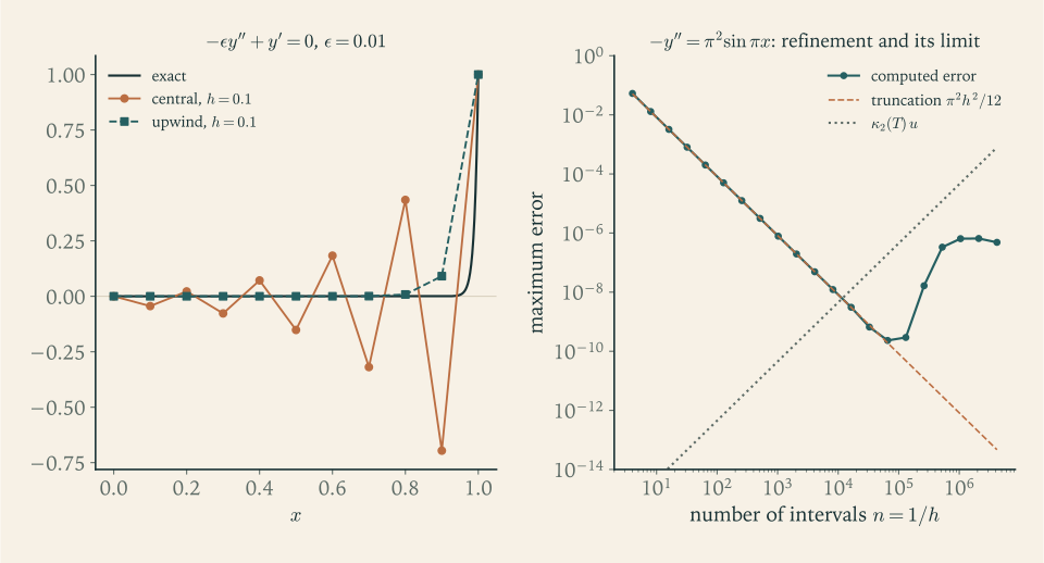
The left panel of Figure 10.1 is this example. Its lesson parallels Section 9.5: a scheme can be formally second-order accurate and still produce nonsense on a grid that does not resolve the fastest scale in the problem, and the symptom is again a sawtooth oscillation.
10.4 Shooting
The second approach works with the nonlinear problem \(y''=g(x,y,y')\) , \(y(a)=\alpha\) , \(y(b)=\beta\) as easily as with a linear one. Replace the far boundary condition by a guessed initial slope \(s\) and solve the initial-value problem
by a method of Chapter 9. Call the resulting value at the far end \(y(b;s)\) . The boundary-value problem is solved when
a scalar equation for \(s\) , to which the secant method or Newton’s method of Chapter 3 applies. Each evaluation of \(F\) costs one integration across the interval. For a linear differential equation \(F\) is an affine function of \(s\) , and two integrations determine its root exactly (Exercise 10.11).
Example 10.4: A nonlinear problem with two solutions
Consider \(y''=\tfrac32y^2\) , \(y(0)=4\) , \(y(1)=1\) . One checks that \(y(x)=4/(1+x)^2\) is a solution, with initial slope \(y'(0)=-8\) . Integrate with the fourth-order Runge–Kutta method and \(h=0.01\) , and apply the secant method to \(F(s)=y(1;s)-1\) starting from \(s=-7\) and \(s=-9\) , where \(F=2.644\) and \(F=-1.958\) . The secant iterates are
and the computed solution agrees with \(4/(1+x)^2\) to within \(10^{-7}\) on the whole interval.
Now start the secant method from \(s=-30\) and \(s=-40\) , where \(F=-2.467\) and \(F=1.861\) . It converges just as readily, to
and the corresponding function is a second, entirely different solution of the same boundary-value problem: it plunges to \(-10.69\) near \(x=0.54\) and climbs back to \(1\) at \(x=1\) . Both computations pass every numerical check. Nothing in either reveals the existence of the other. Whether a nonlinear boundary-value problem has one solution, several, or none is a mathematical question that the numerical method does not answer; what it finds depends on where it starts.
Shooting inherits the accuracy of the initial-value solver and the speed of the root-finder. It also inherits the sensitivity of the initial-value problem, and that can be fatal.
Example 10.5: Shooting fails where differences succeed
The problem \(y''=\lambda^2y\) , \(y(0)=1\) , \(y(1)=e^{-\lambda}\) has the decaying solution \(y=e^{-\lambda x}\) . The initial-value problem with slope \(s\) has the solution \(\cosh\lambda x+(s/\lambda)\sinh\lambda x\) , so
For \(\lambda=10\) this is \(1101\) : an error of \(10^{-12}\) in the slope changes \(y(1)\) by \(10^{-9}\) , and shooting works. For \(\lambda=50\) it is \(5.2\times10^{19}\) , larger than \(1/u\) . Even with the exact slope \(s=-50\) , the rounding errors of the integration excite the growing solution \(e^{50x}\) , and a fourth-order integration with \(4000\) steps returned a value of magnitude about \(2\times10^{4}\) for \(y(1)\) , where the true value is \(1.9\times10^{-22}\) ; the particular number is amplified rounding noise and will differ from machine to machine. No choice of \(s\) representable in double precision gives the right answer.
The boundary-value problem itself is perfectly well conditioned: its solution depends on the boundary values with sensitivity at most \(1\) . The finite-difference scheme, with the term \(\lambda^2h^2\) added to the diagonal of \(T\) , respects that. With \(n=1000\) its maximum error for \(\lambda=50\) is \(3.8\times10^{-5}\) , and with \(n=100\) it is \(3.7\times10^{-3}\) .
This is the distinction of Chapter 1 once more. The problem is well conditioned, and shooting is an unstable algorithm for it, because it passes through an intermediate problem, the initial-value problem, that is violently ill conditioned. Shooting is the method of choice when the differential equation has no rapidly growing solutions in either direction; otherwise use differences, or shoot over short subintervals.
10.5 Evidence that a computed solution is right
In every example so far the exact solution was known and the error could be displayed. In real use it is not, and the question becomes what a careful person does to justify trusting the numbers. The tools have all appeared in earlier chapters, and this section assembles them.
Refine and observe the order. Compute on grids \(h\) , \(h/2\) , \(h/4\) . If the method has order \(p\) and the grids are fine enough, successive differences shrink by \(2^{p}\) , exactly as in Section 6.2:
An observed order equal to the theoretical one is strong evidence that the code is correct and the grid is in the asymptotic regime. An observed order that is wrong means something is wrong: a bug, an unresolved layer, a solution less smooth than assumed, or rounding.
Estimate the error by extrapolation. Once the order is confirmed, \((Y_{h/4}-Y_{h/2})/(2^{p}-1)\) estimates the error of \(Y_{h/4}\) , by the Richardson argument of Section 6.3.
Check with an independent method. Agreement between two methods with different error mechanisms, here differences and shooting, is evidence that neither shares a systematic mistake.
Test the code on a manufactured solution. Choose a smooth function, substitute it into the differential equation to define the right-hand side and boundary values, and verify that the program reproduces it with the expected order (Exercise 10.17).
Example 10.6: A problem with no formula for its solution
Solve \(-y''+(1+x^2)\,y=1\) , \(y(0)=y(1)=0\) by central differences, with \((1+x_j^2)h^2\) added to the diagonal of \(T\) . The computed values at \(x=\tfrac12\) are:
| \(n\) | \(20\) | \(40\) | \(80\) |
|---|---|---|---|
| \(Y(\tfrac12)\) | \(0.110238836627\) | \(0.110257683007\) | \(0.110262401766\) |
The successive differences are \(1.8846\times10^{-5}\) and \(4.7188\times10^{-6}\) , with ratio \(3.994\) , so the observed order is \(\log_23.994=1.998\) : second order, as the theory says. The Richardson estimate of the error of the finest value is \(4.7188\times10^{-6}/3=1.573\times10^{-6}\) , and the extrapolated value is \(0.110263974686\) .
For an independent check, solve the same problem by shooting: the equation is linear, so two fourth-order Runge–Kutta integrations with \(h=0.005\) determine the slope \(y'(0)=0.45562407\) and give \(y(\tfrac12)=0.110263975321\) . The finite-difference value at \(n=80\) differs from this by \(1.5736\times10^{-6}\) , in agreement with the Richardson estimate to four digits, and the extrapolated value differs from it by \(6\times10^{-10}\) . Three separate lines of evidence, the observed order, the error estimate, and an unrelated method, support the statement that \(y(\tfrac12)=0.1102640\) to seven digits. No formula for \(y\) was needed.
Refinement has a limit, and it is the limit that Chapter 1 predicted. The matrix \(T/h^2\) has condition number about \(4n^2/\pi^2\) , so by Section 7.3 rounding errors in solving the system can be amplified by that factor: the computed solution carries a rounding error that grows like \(u/h^2\) while the truncation error falls like \(h^2\) . For the model problem of Example 10.1 the error decreases like \(0.82\,h^2\) down to about \(2\times10^{-10}\) near \(n=65\,000\) , and for larger \(n\) it rises again, erratically, reaching about \(10^{-6}\) at \(n=10^{6}\) . The right panel of Figure 10.1 shows the two regimes, the mirror image of Figure 1.1. The bound \(\kappa u\) overestimates the rounding error considerably here, but the trend is as predicted, and it sets the practical rule: when the observed order collapses on the finest grids, suspect rounding, and stop refining.
Common mistake. Presenting a single computed solution, on a single grid, as the answer. One computation carries no information about its own error. The minimum evidence is a second computation on a refined grid and the difference between the two; the standard is three grids and an observed order. And no amount of refinement evidence addresses the questions that Example 10.4 raised, whether the problem has other solutions, or whether the equations describe the situation they were meant to model. Convergence shows that the equations were solved. It does not show that they were the right equations.
10.6 Choosing a method
The chapters of this book have treated one kind of problem after another. In retrospect the same four questions were asked each time, and they are the questions to ask of any new computation.
How sensitive is the problem? Compute or estimate a condition number before blaming or trusting an algorithm: the relative condition number of a function (Chapter 1), the reciprocal slope at a root (Chapter 2), the Lebesgue constant of a node set (Chapter 4), \(\kappa(A)\) for a linear system or a least-squares problem (Chapters 5 and 7), the growth of perturbations of an initial-value problem (Chapters 9 and 10). An ill-conditioned problem needs better data or a reformulation, not a better solver.
Is the algorithm stable? A stable algorithm gives the exact answer to a nearby problem. Unstable ones have recognizable signatures: subtraction of nearly equal quantities, large multipliers, recurrences run in the growing direction, normal equations, explicit time-stepping beyond the stability limit, shooting against a growing solution.
What is the truncation error and its order? Know the theorem, including its hypotheses on smoothness, and confirm the order experimentally. Higher order pays when the solution is smooth and the accuracy demanded is high; it is wasted, or harmful, on rough data.
What structure can be exploited, and what evidence will be produced? Symmetry, positive definiteness, bandedness, sparsity, periodicity, and smoothness each have a method that uses them. And every computation should end with something checkable: a bracket, a residual together with a condition estimate, an observed order, an agreement between independent methods.
The following table condenses the choices this book supports.
| problem | first choice | when it fails or is too slow | evidence to report |
|---|---|---|---|
| scalar root | safeguarded Newton or Brent | multiple root: expect \(\sqrt u\) accuracy | bracket width, residual, slope |
| function from exact data | cubic spline; Chebyshev interpolation if nodes are free | noisy data: fit instead | error bound or refinement |
| function from noisy data | least squares by QR | ill-conditioned basis: change basis | residual, \(\kappa(A)\) |
| integral | adaptive rule; Gauss if smooth | hidden features: split the interval | two tolerances agree |
| dense linear system | LU with partial pivoting; Cholesky if positive definite | large \(\kappa\) : reformulate | residual and \(\kappa(A)\) |
| large sparse system | conjugate gradients, preconditioned | not positive definite: GMRES | residual history |
| eigenvalues | QR algorithm; power or inverse iteration for one | nonsymmetric: sensitivity | residual, symmetry |
| initial-value problem | adaptive explicit Runge–Kutta | stiff: implicit method | tolerance study |
| boundary-value problem | finite differences | no growing modes: shooting also | observed order, second method |
None of these choices is permanent. Each is a default that the four questions may overturn for a particular problem, and the ability to say why is what distinguishes numerical analysis from the use of numerical software.
Exercises
-
Solve \(-y''=1\) , \(y(0)=y(1)=0\) by finite differences with \(h=\tfrac13\) , compare with the exact solution \(y=\tfrac12x(1-x)\) , and explain why the scheme is exact for this problem on every grid.
Solution
With \(h=\tfrac13\) there are two unknowns, and the equations \((-Y_{j-1}+2Y_j-Y_{j+1})/h^2=1\) with \(Y_0=Y_3=0\) are
\[ 2Y_1-Y_2=\tfrac19,\qquad-Y_1+2Y_2=\tfrac19 . \]By symmetry, or by adding the equations, \(Y_1=Y_2=\tfrac19\) . The exact solution gives \(y(\tfrac13)=\tfrac12\cdot\tfrac13\cdot\tfrac23=\tfrac19\) and the same at \(x=\tfrac23\) . The finite-difference values are exact.
This is no accident of the grid. The local truncation error of the scheme is \(-\tfrac1{12}h^2y''''(\xi_j)\) , and for \(y=\tfrac12x(1-x)\) , a quadratic, \(y''''\equiv0\) . So the exact solution satisfies the difference equations with no defect, the error \(E_j=y(x_j)-Y_j\) satisfies the homogeneous difference equations with zero boundary values, and Lemma 10.2 with \(g=0\) gives \(E_j=0\) for every \(j\) and every \(n\) . More generally the scheme reproduces at the grid points any solution that is a polynomial of degree at most \(3\) . That is a useful first test of a program: on such a problem any error larger than rounding is a bug.
-
Show from the identity at the head of Section 10.1 that the second difference reproduces \(-y''(x_j)\) exactly when \(y\) is a polynomial of degree at most \(3\) , and identify the first power of \(x\) for which it does not.
Answer
The remainder is \(-\tfrac1{12}h^2y''''(\xi_j)\) , which vanishes identically when \(y\) has degree at most \(3\) . For \(y=x^4\) , \(y''''=24\) and the second difference differs from \(-y''(x_j)\) by exactly \(-2h^2\) .
-
Write the finite-difference equations for \(-y''=0\) , \(y(0)=1\) , \(y(1)=3\) with \(n=4\) , showing where the boundary values enter the right-hand side, and verify that the grid values of \(y=1+2x\) satisfy them.
Answer
With \(h=\tfrac14\) and \(f=0\) , multiply by \(h^2\) and move the known boundary values to the right: \(2Y_1-Y_2=1\) , \(-Y_1+2Y_2-Y_3=0\) , \(-Y_2+2Y_3=3\) . The values \(Y=(1.5,2,2.5)\) of \(1+2x\) give \(3-2=1\) , \(-1.5+4-2.5=0\) , and \(-2+5=3\) .
-
Prove that the matrix \(T\) of order \(m\) is positive definite by establishing the identity \(z^{\top}Tz=z_1^2+\sum_{i=1}^{m-1}(z_{i+1}-z_i)^2+z_m^2\) .
Solution
Expand the quadratic form. The diagonal of \(T\) contributes \(2\sum_{i=1}^{m}z_i^2\) and the two off-diagonals contribute \(-2\sum_{i=1}^{m-1}z_iz_{i+1}\) :
\[ z^{\top}Tz=2\sum_{i=1}^{m}z_i^2-2\sum_{i=1}^{m-1}z_iz_{i+1}. \]Now expand the proposed right-hand side: \(\sum_{i=1}^{m-1}(z_{i+1}-z_i)^2=\sum_{i=1}^{m-1}z_{i+1}^2+\sum_{i=1}^{m-1}z_i^2-2\sum_{i=1}^{m-1}z_iz_{i+1}\) . The first two sums together contain every \(z_i^2\) twice except \(z_1^2\) and \(z_m^2\) , which appear once; adding the separate terms \(z_1^2\) and \(z_m^2\) completes them to \(2\sum_{i=1}^{m}z_i^2\) . This proves the identity.
The right-hand side is a sum of squares, so \(z^{\top}Tz\ge0\) . If it is zero, every square vanishes: \(z_1=0\) , and \(z_{i+1}=z_i\) for each \(i\) , so all components are zero. Hence \(z^{\top}Tz>0\) for \(z\ne0\) , and since \(T\) is symmetric it is positive definite. Consequently \(T\) is nonsingular, the finite-difference equations have a unique solution for every right-hand side, Cholesky factorization applies without pivoting, and the conjugate gradient method of Section 8.6 is available.
-
For \(n=4\) compute the inverse of the \(3\times3\) matrix \(T\) , find the \(\infty\) -norm of \((T/h^2)^{-1}\) , and compare with the constant in Lemma 10.2.
Solution
For \(n=4\) ,
\[ T^{-1}=\frac14\begin{pmatrix}3&2&1\\2&4&2\\1&2&3\end{pmatrix}, \]as one checks by multiplying: the first row of \(T\) times the first column of the candidate gives \(\tfrac14(6-2)=1\) , and times the second column gives \(\tfrac14(4-4)=0\) . The absolute row sums of \(T^{-1}\) are \(\tfrac32\) , \(2\) , \(\tfrac32\) , so \(\lVert T^{-1}\rVert_\infty=2\) . Since \((T/h^2)^{-1}=h^2T^{-1}\) with \(h^2=\tfrac1{16}\) ,
\[ \lVert(T/h^2)^{-1}\rVert_\infty=\tfrac1{16}\times2=\tfrac18 . \]Lemma 10.2 asserts that this norm is at most \(\tfrac18\) for every \(n\) , and here the bound is attained. The reason is visible in the proof: the comparison function \(W_j=\tfrac12x_j(1-x_j)\) is the exact solution of the difference equations with right-hand side \(1\) , it has maximum \(\tfrac18\) at \(x=\tfrac12\) , and \(\tfrac12\) is a grid point when \(n\) is even. All entries of \(T^{-1}\) are positive, which is the matrix form of the maximum principle: nonnegative data give a nonnegative solution.
-
From the errors in Example 10.2 compute the observed orders, and use the fitted error \(0.82\,h^2\) to find the number of intervals needed for an error below \(10^{-6}\) .
Answer
The orders are \(\log_2(5.303/1.295)=2.03\) , then \(2.01\) , \(2.00\) , \(2.00\) . Requiring \(0.82\,h^2\le10^{-6}\) gives \(n=1/h\ge\sqrt{0.82\times10^{6}}=905.5\) , so \(906\) intervals.
-
The boundary condition at \(x=1\) is changed to \(y'(1)=\gamma\) . Using a fictitious grid value \(Y_{n+1}\) and the central difference \((Y_{n+1}-Y_{n-1})/(2h)=\gamma\) , derive the equation that replaces \(Y_n=\beta\) , and state the order of accuracy of the resulting scheme.
Hint
Write the difference equation at \(j=n\) , which involves \(Y_{n+1}\) , and eliminate \(Y_{n+1}=Y_{n-1}+2h\gamma\) . The result is \((-2Y_{n-1}+2Y_n)/h^2=f(x_n)+2\gamma/h\) . Both the difference equation and the boundary approximation are second-order accurate, and so is the scheme.
-
For \(-\epsilon y''+y'=0\) discretized with central differences on a uniform grid, show that the difference equation has the solutions \(Y_j=A+Br^{j}\) with \(r=(1+P)/(1-P)\) and \(P=h/(2\epsilon)\) , and deduce that the numerical solution oscillates if and only if \(P>1\) .
Solution
The central scheme at an interior point is
\[ -\epsilon\,\frac{Y_{j-1}-2Y_j+Y_{j+1}}{h^2}+\frac{Y_{j+1}-Y_{j-1}}{2h}=0 . \]Multiply by \(h^2/\epsilon\) and write \(P=h/(2\epsilon)\) : \(-(1+P)Y_{j-1}+2Y_j-(1-P)Y_{j+1}=0\) . Substituting \(Y_j=r^{j}\) and dividing by \(r^{j-1}\) gives the quadratic
\[ (1-P)\,r^2-2r+(1+P)=0 . \]One root is \(r=1\) , since \((1-P)-2+(1+P)=0\) . The product of the roots is \((1+P)/(1-P)\) , so the other root is \(r=(1+P)/(1-P)\) , provided \(P\ne1\) . The difference equation is linear of second order, so its general solution is \(Y_j=A\cdot1^{j}+Br^{j}=A+Br^{j}\) , and the boundary conditions \(Y_0=0\) , \(Y_n=1\) give \(Y_j=(r^{j}-1)/(r^{n}-1)\) .
If \(P<1\) then \(r>1\) and \(Y_j\) increases monotonically, like the true solution; indeed \(r=e^{h/\epsilon}\bigl(1+O(P^2)\bigr)\) , so \(r^{j}\approx e^{x_j/\epsilon}\) . If \(P>1\) then \(r<0\) and \(r^{j}\) alternates in sign: the numerical solution oscillates from one grid point to the next, with amplitude growing like \(\lvert r\rvert^{j}\) . So oscillation occurs exactly when \(P>1\) , that is, when \(h>2\epsilon\) . For \(\epsilon=0.01\) and \(h=0.1\) , \(P=5\) and \(r=-1.5\) , as in Example 10.3.
-
Show that the upwind scheme for \(-\epsilon y''+y'=0\) is identical to the central scheme applied to the same equation with \(\epsilon\) replaced by \(\epsilon+\tfrac12h\) , and use this to explain both its stability and its smearing of the boundary layer.
Solution
The upwind scheme is
\[ -\epsilon\,\frac{Y_{j-1}-2Y_j+Y_{j+1}}{h^2}+\frac{Y_j-Y_{j-1}}{h}=0 . \]The one-sided difference can be split into a central difference and a second difference:
\[ \frac{Y_j-Y_{j-1}}{h}=\frac{Y_{j+1}-Y_{j-1}}{2h}-\frac h2\cdot\frac{Y_{j-1}-2Y_j+Y_{j+1}}{h^2}, \]as one verifies by putting the right side over the denominator \(2h\) . Substituting,
\[ -\Bigl(\epsilon+\frac h2\Bigr)\frac{Y_{j-1}-2Y_j+Y_{j+1}}{h^2}+\frac{Y_{j+1}-Y_{j-1}}{2h}=0, \]which is the central scheme for \(-\tilde\epsilon\,y''+y'=0\) with \(\tilde\epsilon=\epsilon+\tfrac12h\) .
Stability. By Exercise 10.8 the central scheme oscillates when \(h/(2\tilde\epsilon)>1\) . Here \(h/(2\tilde\epsilon)=h/(2\epsilon+h)<1\) for every \(h>0\) , so the upwind scheme never oscillates. Smearing. The scheme is solving, to second order, a problem whose diffusion coefficient is \(\epsilon+\tfrac12h\) , and whose boundary layer therefore has width of order \(\epsilon+\tfrac12h\) instead of \(\epsilon\) . On a coarse grid the artificial diffusion \(\tfrac12h\) dominates and the layer is spread over a grid cell or two. The upwind scheme is a first-order approximation of the original problem and a second-order approximation of a nearby, more diffusive one.
-
A student computes the central-difference solution of \(-0.01\,y''+y'=0\) on a grid with \(h=0.1\) , sees oscillations, attributes them to rounding error, and repeats the computation in higher precision. Predict the outcome, give the correct diagnosis, and state two remedies.
Answer
Higher precision changes nothing: the oscillating values are the exact solution of the difference equations, \(Y_j=A+B(-1.5)^{j}\) , not a product of rounding. The grid has \(h/(2\epsilon)=5>1\) and does not resolve the layer. Remedies: refine to \(h<2\epsilon=0.02\) , at least near \(x=1\) , with a nonuniform grid if the cost matters; or use the upwind scheme and accept first-order accuracy and a smeared layer.
-
Solve \(y''=y\) , \(y(0)=0\) , \(y(1)=1\) by linear shooting: integrate exactly with slopes \(s=0\) and \(s=1\) , combine the two solutions, and compare the resulting slope with the exact one.
Solution
The differential equation \(y''=y\) is linear, so the solution of the initial-value problem with \(y(0)=0\) , \(y'(0)=s\) depends linearly on \(s\) .
First shot, \(s=0\) : the solution is \(y\equiv0\) , so \(y(1;0)=0\) . Second shot, \(s=1\) : the solution with \(y(0)=0\) and \(y'(0)=1\) is \(\sinh x\) , so \(y(1;1)=\sinh1=1.1752\) .
By linearity \(y(x;s)=y(x;0)+s\bigl(y(x;1)-y(x;0)\bigr)=s\sinh x\) , and the shooting function is \(F(s)=s\sinh1-1\) . Its root is
\[ s=1/\sinh1=0.85092 , \]and the solution of the boundary-value problem is \(y(x)=\sinh x/\sinh1\) , which is the exact solution; its slope at \(0\) is \(1/\sinh1\) , the value found. Two integrations sufficed, with no iteration, because \(F\) is affine. In a numerical setting the two shots would be computed by a Runge–Kutta method and the same combination formed; the only errors would be those of the integrations. The sensitivity here is \(\partial y(1;s)/\partial s=\sinh1\approx1.2\) , so shooting is perfectly well conditioned for this problem.
-
For \(y''=400\,y\) , \(y(0)=1\) , \(y(1)=e^{-20}\) , compute the sensitivity \(\partial y(1;s)/\partial s\) of the shooting function, and state how many digits of \(y(1)\) can be controlled through \(s\) in double precision.
Answer
\(\partial y(1;s)/\partial s=\sinh(20)/20=1.2\times10^{7}\) . The slope \(s\approx-20\) can be specified in double precision only to about \(20u\approx2\times10^{-15}\) , which moves \(y(1)\) by about \(3\times10^{-8}\) . The target \(y(1)=e^{-20}=2.1\times10^{-9}\) is smaller than that, so shooting controls no digit of it: the far boundary value is fixed to an absolute accuracy of about \(10^{-8}\) at best.
-
In Example 10.4, verify the first secant iterate from the two starting values and the two given values of \(F\) , and explain why convergence to \(-8.00000004\) instead of \(-8\) is not a failure of the secant method.
Answer
\(s_2=-9-(-1.958)\dfrac{-9-(-7)}{-1.958-2.644}=-9+\dfrac{3.916}{4.602}=-8.1491\) . The secant method finds the root of the function \(F\) it is given, and that \(F\) is computed with a Runge–Kutta integration of step \(0.01\) , whose discretization error shifts the root by \(4\times10^{-8}\) from the true slope \(-8\) . A finer integration step moves the limit closer to \(-8\) .
-
The boundary-value problem of Example 10.4 is to be solved by finite differences and Newton’s method for the resulting nonlinear system. Describe the system and the structure of its Jacobian, and explain what determines which of the two solutions is found.
Hint
The unknowns are \(Y_1,\dots,Y_{n-1}\) and the equations are \((Y_{j-1}-2Y_j+Y_{j+1})/h^2-\tfrac32Y_j^2=0\) . Differentiate equation \(j\) with respect to \(Y_{j-1}\) , \(Y_j\) , \(Y_{j+1}\) to see that the Jacobian is tridiagonal, so each Newton step costs order \(n\) . Newton’s method converges locally; which solution it reaches is decided by the starting vector, for instance the grid values of a guess that stays positive or of one that dips well below zero.
-
From the three values in Example 10.6, compute the observed order, the Richardson error estimate for the finest grid, and the extrapolated value, showing the arithmetic.
Solution
Let \(a=0.110238836627\) , \(b=0.110257683007\) , \(c=0.110262401766\) be the values for \(n=20,40,80\) .
Order. The differences are \(b-a=1.884638\times10^{-5}\) and \(c-b=4.718759\times10^{-6}\) . Their ratio is \(3.9939\) , and \(\log_23.9939=1.998\) . The method behaves as a second-order method on these grids.
Error estimate. With \(p=2\) , the error of the finest value is estimated by \((c-b)/(2^2-1)=4.718759\times10^{-6}/3\) , which is \(1.5729\times10^{-6}\) .
Extrapolation. Adding the estimate to \(c\) gives \(0.110262401766+0.000001572920\) , that is, \(0.110263974686\) .
The reasoning is that of Section 6.3: if \(Y(h)=y+Ch^2+O(h^4)\) , then \(c-b=C\bigl((h/2)^2-(h/4)^2\bigr)+\cdots=3C(h/4)^2+\cdots\) , so \((c-b)/3\) is the leading error \(C(h/4)^2\) of \(c\) with its sign, and \(c+(c-b)/3\) has error \(O(h^4)\) . The ratio \(3.9939\) being so close to \(4\) is what licenses the use of \(p=2\) ; had it been \(3.5\) or \(5\) , the estimate would not be trustworthy.
-
Explain why the finite-difference error for the model problem cannot be reduced much below \(10^{-10}\) in double precision however fine the grid, by balancing the truncation error against a rounding error proportional to \(u/h^2\) , and compare the predicted optimal \(n\) with the observation in Section 10.5.
Hint
Set \(0.82\,h^2=cu/h^2\) , so \(h^4=cu/0.82\) . With the pessimistic \(c=4/\pi^2\) from \(\kappa_2(T)u\) this gives \(n\approx10^{4}\) and a best error near \(10^{-8}\) ; the observed optimum, \(n\approx6.5\times10^{4}\) with error \(2\times10^{-10}\) , corresponds to \(c\approx4\times10^{-4}\) , about a thousand times smaller. Either way the best error is of order \(\sqrt u\) times a modest factor, as for the second difference in Exercise 1.12.
-
To test a program that solves \(-y''+y=f\) with zero boundary values, choose the manufactured solution \(y(x)=x(1-x)e^{x}\) . Compute the right-hand side \(f\) it requires, and describe the experiment and the outcome that would confirm the program.
Answer
\(y'=(1-x-x^2)e^{x}\) and \(y''=(-3x-x^2)e^{x}\) , so \(f=-y''+y=(3x+x^2)e^{x}+(x-x^2)e^{x}=4xe^{x}\) . Run the program with this \(f\) on grids \(n=20,40,80,160\) , compute the maximum grid error against \(x(1-x)e^{x}\) , and confirm that it falls by a factor of four per doubling. Any other observed order indicates an error in the program.
-
For each task name the method you would use from this book and one piece of evidence you would report: (a) a \(50\times50\) symmetric positive definite system; (b) the integral of a smooth function with a sharp peak at an unknown location; (c) the smallest eigenvalue of a large sparse symmetric matrix; (d) a table of twenty accurate, equally spaced values to be interpolated.
Answer
(a) Cholesky factorization; report the residual and a condition estimate. (b) Adaptive quadrature started from a subdivision fine enough to detect the peak; report agreement at two tolerances. (c) Inverse iteration with shift near zero, or a Krylov eigensolver; report \(\lVert Ax-\mu x\rVert_2\) , which by Theorem 8.2 bounds the eigenvalue error. (d) A not-a-knot cubic spline; report the change when every other point is omitted.
-
The eigenvalue problem \(-y''=\lambda y\) , \(y(0)=y(1)=0\) has eigenvalues \(\lambda_k=k^2\pi^2\) . Use Exercise 8.19 to give the eigenvalues of the finite-difference matrix \(T/h^2\) , compute the smallest for \(n=10\) , and show that its relative error is approximately \(\pi^2h^2/12\) .
Solution
The matrix of the discrete problem is \(T/h^2\) of order \(n-1\) . By Exercise 8.19, with \(n-1\) in place of \(n\) so that \(\pi/(n-1+1)=\pi h\) , its eigenvalues are
\[ \lambda_k^{(h)}=\frac{2-2\cos(k\pi h)}{h^2},\qquad k=1,\dots,n-1 , \]with eigenvectors that are the grid values of the exact eigenfunctions \(\sin k\pi x\) .
For \(n=10\) and \(k=1\) : \(\lambda_1^{(h)}=100\,(2-2\cos(\pi/10))\) , which is \(9.7887\) , against the exact \(\pi^2=9.8696\) . The relative error is \(8.2\times10^{-3}\) .
To explain it, use \(2-2\cos\theta=\theta^2-\tfrac1{12}\theta^4+O(\theta^6)\) with \(\theta=k\pi h\) :
\[ \lambda_k^{(h)}=k^2\pi^2\Bigl(1-\tfrac1{12}k^2\pi^2h^2+O(h^4)\Bigr). \]The relative error of the \(k\) -th eigenvalue is therefore about \(k^2\pi^2h^2/12\) . For \(k=1\) and \(h=0.1\) this is \(\pi^2/1200=8.2\times10^{-3}\) , matching the computation. The formula also shows that the error grows like \(k^2\) : the low eigenvalues are approximated to second order, while those with \(k\) comparable to \(n\) are not approximated at all. A grid resolves only the modes that vary slowly on its scale.
-
Discretizing the heat equation in space by the scheme of Section 10.1 gives the system \(Y'(t)=-\tfrac1{h^2}TY(t)\) . Using the eigenvalues of \(T\) , find the stability limit on the time step of Euler’s method, evaluate it for \(h=0.01\) , and say why the system is stiff.
Answer
The eigenvalues of \(-T/h^2\) are \(-(2-2\cos k\pi h)/h^2\) , ranging from about \(-\pi^2\) to about \(-4/h^2\) . Euler’s method needs \(\Delta t\cdot4/h^2\le2\) , that is, \(\Delta t\le\tfrac12h^2\) , which is \(5\times10^{-5}\) for \(h=0.01\) . The solution, after a brief transient, decays at the slow rate \(\pi^2\approx10\) , on a time scale of \(0.1\) , while stability is dictated by the fastest mode with rate \(4\times10^{4}\) : the ratio of scales is \(4000\) and grows as the grid is refined. The system is stiff, and an implicit method, with a tridiagonal solve per step, removes the restriction.