A square grid of \(1000\times1000\) points carries one unknown per point, a million in all, and each equation couples a point to its four neighbours. The matrix has \(10^{12}\) entries, of which five million are nonzero. Storing it as a full array is out of the question, and elimination, even exploiting the band, would create billions of new nonzero entries inside the band and need about \(10^{12}\) operations. What can be done cheaply with such a matrix is to multiply it by a vector: five million multiplications, and no storage beyond the nonzeros.
So the question of this chapter is what can be computed about a matrix using only products \(Av\) . The answer covers two problems that look different and are closely related. One is the eigenvalue problem, which cannot be solved by any finite procedure and is therefore iterative by nature. The other is the solution of \(Ax=b\) for large sparse \(A\) , where iteration replaces factorization. In both, the speed of convergence is governed by the eigenvalues of some matrix, and in both, the analysis of Chapter 3 returns in matrix form: an iteration \(x_{k+1}=Gx_k+c\) is a fixed-point iteration, and whether it contracts is decided by the spectrum of \(G\) .
Throughout, eigenvalues and eigenvectors are used as defined in Linear Algebra (math.linear-algebra.eigenvector-as-steady-direction), together with one theorem proved there: a real symmetric matrix has real eigenvalues and an orthonormal basis of eigenvectors.
8.1 Power iteration
Multiply a vector by \(A\) repeatedly. Its components along the eigenvectors of \(A\) are multiplied by the corresponding eigenvalues each time, and the component belonging to the eigenvalue of largest magnitude outgrows the others. Normalizing at each step to avoid overflow gives power iteration:
The natural eigenvalue estimate that accompanies a vector \(x\) is its Rayleigh quotient \(R(x)=x^{\top}Ax/x^{\top}x\) .
Theorem 8.1 (convergence of power iteration). Let \(A\) have a basis of eigenvectors \(v_1,\dots,v_n\) with eigenvalues satisfying \(\lvert\lambda_1\rvert>\lvert\lambda_2\rvert\ge\dots\ge\lvert\lambda_n\rvert\) , and let \(x_0=\sum_ic_iv_i\) with \(c_1\ne0\) . Then the direction of \(x_k\) converges to that of \(v_1\) , with error of order \(\lvert\lambda_2/\lambda_1\rvert^{k}\) . If \(A\) is symmetric, the Rayleigh quotients satisfy \(\lvert R(x_k)-\lambda_1\rvert=O\bigl(\lvert\lambda_2/\lambda_1\rvert^{2k}\bigr)\) .
Proof. The iterate \(x_k\) is a scalar multiple of \(A^{k}x_0=\lambda_1^{k}\bigl(c_1v_1+\sum_{i\ge2}c_i(\lambda_i/\lambda_1)^{k}v_i\bigr)\) , and each ratio \((\lambda_i/\lambda_1)^{k}\) is at most \(\lvert\lambda_2/\lambda_1\rvert^{k}\) in magnitude, which proves the first claim. For symmetric \(A\) take the \(v_i\) orthonormal and write a unit vector as \(x=\cos\theta\,v_1+\sin\theta\,w\) with \(w\) a unit vector orthogonal to \(v_1\) . Then \(Av_1=\lambda_1v_1\) is orthogonal to \(w\) , so \(R(x)=\lambda_1\cos^2\theta+(w^{\top}Aw)\sin^2\theta\) and
The eigenvalue error is proportional to the square of the angle between \(x\) and \(v_1\) , and that angle is of order \(\lvert\lambda_2/\lambda_1\rvert^{k}\) .
Each step costs one multiplication by \(A\) . The hypotheses mark the limits of the method. If two eigenvalues share the largest magnitude, for instance \(\lambda\) and \(-\lambda\) , the iterates need not converge. If \(\lvert\lambda_2\rvert\) is close to \(\lvert\lambda_1\rvert\) , convergence is slow. And the method finds one eigenpair only, the dominant one.
Example 8.1: Power iteration on a symmetric matrix
Let
whose eigenvalues are \(3+\sqrt3=4.7320508\) , \(3\) , and \(3-\sqrt3=1.2679492\) . Start from \(x_0=(1,1,1)/\sqrt3\) .
| \(k\) | \(x_k\) | \(R(x_k)\) | \(\lambda_1-R(x_k)\) |
|---|---|---|---|
| \(0\) | \((0.5774,\ 0.5774,\ 0.5774)\) | \(4.3333333\) | \(3.99\times10^{-1}\) |
| \(1\) | \((0.6509,\ 0.6509,\ 0.3906)\) | \(4.6271186\) | \(1.05\times10^{-1}\) |
| \(2\) | \((0.7001,\ 0.6441,\ 0.3081)\) | \(4.6941176\) | \(3.79\times10^{-2}\) |
| \(5\) | \((0.7666,\ 0.5984,\ 0.2331)\) | \(4.7296199\) | \(2.43\times10^{-3}\) |
| \(10\) | \((0.7865,\ 0.5796,\ 0.2135)\) | \(4.7320253\) | \(2.55\times10^{-5}\) |
| \(20\) | \((0.7887,\ 0.5774,\ 0.2113)\) | \(4.7320508\) | \(2.81\times10^{-9}\) |
The dominant eigenvector is \((0.7887,0.5774,0.2113)\) . The ratio \(\lambda_2/\lambda_1\) is \(3/4.732=0.634\) , so the vector error falls by that factor per step, a digit every five steps: at \(k=20\) the vector is correct to about four digits. The eigenvalue error falls by \(0.634^2=0.402\) per step, and the observed ratios of successive eigenvalue errors settle at \(0.402\) . After twenty steps the eigenvalue has eight correct digits and the eigenvector four, exactly the two-to-one relation the theorem describes.
8.2 Shifts, inverse iteration, and what a residual certifies
Power iteration can be aimed at other eigenvalues by applying it to a function of \(A\) . If \(A\) has eigenpairs \((\lambda_i,v_i)\) and \(\mu\) is not an eigenvalue, then \((A-\mu I)^{-1}\) has the same eigenvectors with eigenvalues \(1/(\lambda_i-\mu)\) . The largest of these in magnitude belongs to the \(\lambda_i\) closest to \(\mu\) . Inverse iteration with shift \(\mu\) is power iteration for \((A-\mu I)^{-1}\) :
The inverse is not formed. The matrix \(A-\mu I\) is factored once, as in Chapter 7, and each step is a pair of triangular solves. If \(\lambda_J\) is the eigenvalue nearest \(\mu\) and \(\lambda_K\) the next nearest, the convergence ratio is \(\lvert\lambda_J-\mu\rvert/\lvert\lambda_K-\mu\rvert\) , which a good shift makes very small. The apparent paradox that \(A-\mu I\) is nearly singular when \(\mu\) is a good shift is harmless: the error made in solving the ill-conditioned system lies almost entirely in the direction of the wanted eigenvector.
Taking the best available shift at every step, \(\mu_k=R(x_k)\) , gives Rayleigh quotient iteration. It needs a new factorization per step, and for symmetric matrices it converges cubically: the number of correct digits triples each time. We state this without proof.
Example 8.2: Inverse iteration and Rayleigh quotient iteration
For the matrix of Example 8.1 take the shift \(\mu=1\) , nearest to the eigenvalue \(\lambda_3=1.2679492\) . The predicted ratio is \((1.268-1)/(3-1)=0.134\) for the vector and \(0.134^2=0.018\) for the Rayleigh quotient. From \(x_0=(1,1,1)/\sqrt3\) the Rayleigh quotients are
| \(k\) | \(1\) | \(2\) | \(3\) | \(4\) | \(5\) |
|---|---|---|---|---|---|
| \(R(x_k)\) | \(1.5454545\) | \(1.2702703\) | \(1.2679745\) | \(1.2679496\) | \(1.2679492\) |
| \(R(x_k)-\lambda_3\) | \(2.78\times10^{-1}\) | \(2.32\times10^{-3}\) | \(2.53\times10^{-5}\) | \(3.70\times10^{-7}\) | \(6.20\times10^{-9}\) |
Each step gains nearly two digits, with successive error ratios approaching \(0.018\) . Five steps of inverse iteration achieve what power iteration needed twenty for, and they find an eigenvalue that power iteration could not find at all.
Rayleigh quotient iteration from the same \(x_0\) produces the shifts \(4.3333333\) , \(4.7074172\) , \(4.7320463\) , \(4.7320508\) , with errors \(3.99\times10^{-1}\) , \(2.46\times10^{-2}\) , \(4.54\times10^{-6}\) , and then rounding level. The last useful step cubed an error of about \(2\times10^{-2}\) .
When an iteration is stopped, the quantity at hand is the eigen-residual \(Ax-\mu x\) . For symmetric matrices it bounds the error of the eigenvalue directly, with no condition number.
Theorem 8.2 (residual bound for symmetric matrices). Let \(A\) be symmetric, \(x\) a unit vector, and \(\mu\) a real number. Then \(A\) has an eigenvalue \(\lambda\) with
Proof. Expand \(x=\sum_ic_iv_i\) in an orthonormal basis of eigenvectors, so that \(\sum_ic_i^2=1\) . Then \(Ax-\mu x=\sum_i(\lambda_i-\mu)c_iv_i\) and
For the starting vector of the examples, \(\mu=R(x_0)=4.3333\) and \(\lVert Ax_0-\mu x_0\rVert_2=0.943\) , so some eigenvalue lies within \(0.943\) of \(4.3333\) ; in fact \(4.732\) does, at distance \(0.399\) . The theorem is the eigenvalue counterpart of Corollary 7.7 with \(\kappa=1\) : eigenvalues of symmetric matrices are perfectly conditioned. Without symmetry the statement is false and eigenvalues can be extremely sensitive.
Example 8.3: A nonsymmetric matrix with fragile eigenvalues
The upper triangular matrix
has eigenvalues \(1\) and \(1.001\) . Change the zero in the lower left corner to \(10^{-6}\) . The eigenvalues become the roots of \((\lambda-1)(\lambda-1.001)=10^{-3}\) , which are \(0.96887\) and \(1.03213\) : a perturbation of size \(10^{-6}\) has moved each eigenvalue by \(0.031\) , an amplification of thirty thousand. For a symmetric matrix the eigenvalues would have moved by at most \(10^{-6}\) . The eigenvectors of \(B\) are nearly parallel, and that near-dependence is what makes its eigenvalues ill conditioned. A small residual for a nonsymmetric eigenproblem certifies, as in Chapter 7, only that the computed pair is exact for a nearby matrix.
8.3 All the eigenvalues: the QR algorithm
Library routines for the full eigenvalue problem use neither determinants nor the characteristic polynomial, whose roots are hopelessly sensitive to its coefficients (recall Example 2.3). They use the QR algorithm. Starting from \(A_0=A\) , factor and recombine in the opposite order:
with \(Q_k\) orthogonal and \(R_k\) upper triangular as in Theorem 5.8. Since \(R_k=Q_k^{\top}A_k\) , the new matrix is \(A_{k+1}=Q_k^{\top}A_kQ_k\) : it is similar to \(A_k\) and has the same eigenvalues, and symmetry is preserved. The iteration is power iteration applied to a whole basis at once, with the QR factorization keeping the basis orthonormal. The convergence theorem, which we quote without proof, needs two hypotheses. Suppose \(A=X\Lambda X^{-1}\) with eigenvalues of distinct magnitudes, ordered so that \(\lvert\lambda_1\rvert>\dots>\lvert\lambda_n\rvert\) , and suppose that all leading principal minors of \(X^{-1}\) are nonzero, which is the matrix form of the requirement in Theorem 8.1 that the starting vector have a component along \(v_1\) . Then the matrices \(A_k\) converge to upper triangular form, diagonal if \(A\) is symmetric, with the eigenvalues on the diagonal in decreasing order of magnitude, and the entry in position \((i+1,i)\) tends to zero like \(\lvert\lambda_{i+1}/\lambda_i\rvert^{k}\) . The second hypothesis holds for all but exceptional matrices, and it cannot be dropped: for the diagonal matrix with entries \(1\) and \(2\) the factorization is \(Q=I\) , \(R=A\) , so every \(A_k\) equals \(A\) and the eigenvalues stay in increasing order for ever.
Example 8.4: QR iteration on the matrix of Example 8.1
| \(k\) | diagonal of \(A_k\) | magnitude of entry \((2,1)\) | magnitude of entry \((3,2)\) |
|---|---|---|---|
| \(0\) | \(4,\ 3,\ 2\) | \(1\) | \(1\) |
| \(1\) | \(4.4118,\ 3.1535,\ 1.4348\) | \(0.6910\) | \(0.5378\) |
| \(5\) | \(4.7224,\ 3.0095,\ 1.2681\) | \(0.1291\) | \(0.0171\) |
| \(10\) | \(4.7319,\ 3.0001,\ 1.2679\) | \(0.0133\) | \(2.31\times10^{-4}\) |
| \(20\) | \(4.7321,\ 3.0000,\ 1.2679\) | \(1.39\times10^{-4}\) | \(4.19\times10^{-8}\) |
The diagonal converges to all three eigenvalues at once. The off-diagonal entries decay at the predicted rates: successive ratios of the \((2,1)\) entry approach \(\lambda_2/\lambda_1=0.634\) , and those of the \((3,2)\) entry approach \(\lambda_3/\lambda_2=0.423\) .
As described, the method is too slow and too expensive, with a full factorization per step and linear convergence. The practical algorithm adds three refinements, none of which changes the idea. The matrix is first reduced by orthogonal similarity transformations to Hessenberg form, zero below the first subdiagonal, which is tridiagonal in the symmetric case; QR steps preserve this form and then cost order \(n^2\) , or order \(n\) for tridiagonal matrices. Shifts are used, as in Section 8.2, so that the last subdiagonal entry converges quadratically or cubically instead of linearly. And when that entry is negligible the last eigenvalue is accepted and the problem deflates to one of smaller order. The result finds all eigenvalues of a dense matrix in about \(10n^3\) operations and is backward stable.
8.4 Solving linear systems by iteration
Return to \(Ax=b\) with \(A\) large and sparse. Split the matrix as \(A=M-N\) with \(M\) nonsingular and easy to solve with. Then \(Ax=b\) is equivalent to \(Mx=Nx+b\) , which suggests the iteration
An iteration of this form, with \(G\) and \(c\) fixed, is called stationary. The solution \(x\) is a fixed point, and subtracting \(x=Gx+c\) gives the error recursion \(e_{k+1}=Ge_k\) , so \(e_k=G^{k}e_0\) .
Theorem 8.3 (convergence of stationary iterations). The iteration \(x_{k+1}=Gx_k+c\) converges to the fixed point for every starting vector if and only if the spectral radius \(\rho(G)=\max_i\lvert\lambda_i(G)\rvert\) is less than \(1\) . In particular it converges if \(\lVert G\rVert<1\) in some induced norm, and then \(\lVert e_k\rVert\le\lVert G\rVert^{k}\lVert e_0\rVert\) .
Proof. If \(\lVert G\rVert<1\) then \(\lVert e_k\rVert=\lVert G^{k}e_0\rVert\le\lVert G\rVert^{k}\lVert e_0\rVert\to0\) . For any eigenpair, \(\lvert\lambda\rvert\lVert v\rVert=\lVert Gv\rVert\le\lVert G\rVert\lVert v\rVert\) , so \(\rho(G)\le\lVert G\rVert\) in every induced norm. If \(\rho(G)\ge1\) , choose \(e_0\) to be an eigenvector, or the real part of one, for an eigenvalue of magnitude at least \(1\) ; then \(G^{k}e_0\) does not tend to zero. Finally, if \(G\) has a basis of eigenvectors and \(\rho(G)<1\) , expanding \(e_0=\sum c_iv_i\) gives \(e_k=\sum c_i\lambda_i^{k}v_i\to0\) . For matrices without a basis of eigenvectors the same conclusion holds, by an argument using the Jordan form that we omit.
The theorem is Theorem 3.3 for linear maps: the derivative of \(x\mapsto Gx+c\) is \(G\) everywhere, and the role of \(\lvert g'(r)\rvert\) is played by \(\rho(G)\) . Asymptotically the error is multiplied by \(\rho(G)\) per iteration, so a reduction by the factor \(10^{-d}\) takes about \(d/\log_{10}(1/\rho(G))\) iterations. A method with \(\rho=0.99\) needs \(229\) iterations per digit.
8.5 Jacobi and Gauss–Seidel iterations
Write \(A=D+L+U\) , with \(D\) the diagonal of \(A\) , \(L\) its strictly lower triangular part, and \(U\) its strictly upper triangular part. The two classical choices of splitting are these.
The Jacobi iteration takes \(M=D\) . Each equation is solved for its own diagonal unknown using the old values of all the others:
The Gauss–Seidel iteration takes \(M=D+L\) . The equations are processed in order, and each new component is used as soon as it has been computed:
Both cost about one multiplication by \(A\) per sweep. Their iteration matrices are \(G_J=-D^{-1}(L+U)\) and \(G_{GS}=-(D+L)^{-1}U\) .
Theorem 8.4 (convergence for strictly diagonally dominant matrices). If \(\lvert a_{ii}\rvert>\sum_{j\ne i}\lvert a_{ij}\rvert\) for every \(i\) , the Jacobi and Gauss–Seidel iterations both converge for every starting vector.
Proof. For Jacobi, row \(i\) of \(G_J\) has entries \(-a_{ij}/a_{ii}\) for \(j\ne i\) , so \(\lVert G_J\rVert_\infty=\max_i\sum_{j\ne i}\lvert a_{ij}\rvert/\lvert a_{ii}\rvert<1\) , and Theorem 8.3 applies. The Gauss–Seidel case is Exercise 8.11.
Two further facts are quoted without proof. Gauss–Seidel converges for every symmetric positive definite matrix. And for tridiagonal matrices, among others, \(\rho(G_{GS})=\rho(G_J)^2\) : one Gauss–Seidel sweep is worth two Jacobi sweeps.
Example 8.5: Both iterations on a small system
Solve
whose solution is \(x=(1,2,3)\) , starting from \(x^{(0)}=0\) . The matrix is strictly diagonally dominant with \(\lVert G_J\rVert_\infty=\tfrac12\) .
Jacobi: the first sweep gives \(x^{(1)}=(2/4,\,4/4,\,10/4)=(0.5,\,1,\,2.5)\) , and the second \(x^{(2)}=\bigl((2+1)/4,\,(4+0.5+2.5)/4,\,(10+1)/4\bigr)=(0.75,\,1.75,\,2.75)\) . Continuing, the maximum errors at sweeps \(1\) to \(8\) are
Over two sweeps the error falls by \(\tfrac18\) , a rate of \(\sqrt{1/8}=0.3536\) per sweep, and indeed \(\rho(G_J)=\sqrt2/4=0.3536\) .
Gauss–Seidel: in the first sweep \(x_1=2/4=0.5\) , then \(x_2=(4+0.5)/4=1.125\) using the new \(x_1\) , then \(x_3=(10+1.125)/4=2.78125\) . The maximum errors at sweeps \(1\) to \(6\) are
falling by the factor \(\tfrac18=0.125=\rho(G_J)^2\) each sweep. Six Gauss–Seidel sweeps do better than eight Jacobi sweeps did.
On small well-conditioned systems these methods are pleasant. On the problems they were invented for, they are slow. The model problem is the tridiagonal matrix \(T_n\) of Example 7.7, of order \(n\) , with \(2\) on the diagonal and \(-1\) beside it. Its eigenvalues are \(2-2\cos\bigl(j\pi/(n+1)\bigr)\) for \(j=1,\dots,n\) (Exercise 8.19), so
For \(n=100\) this is \(\rho(G_J)=0.99952\) : a reduction of the error by \(10^{-6}\) takes \(28\,554\) Jacobi sweeps, or half that many Gauss–Seidel sweeps. The number of sweeps grows like \(n^2\) , in proportion to the condition number. Refining a grid makes the systems both larger and harder.
Common mistake. Judging an iterative solver by the size of the last update \(\lVert x_{k+1}-x_k\rVert\) . For a slowly convergent iteration the update is small because progress is slow, not because the answer is near: with error ratio \(\rho\) the remaining error is about \(\rho/(1-\rho)\) times the last update, which for \(\rho=0.9995\) is a factor of \(2000\) . Monitor the residual \(b-Ax_k\) , which costs one matrix product, and remember Corollary 7.7: even a small relative residual bounds the relative error only after multiplication by \(\kappa(A)\) .
8.6 Conjugate gradients
For symmetric positive definite matrices there is a method of a different kind, which adapts to the right-hand side and whose cost grows like \(\sqrt{\kappa}\) instead of \(\kappa\) .
Let \(A\) be symmetric positive definite and define \(\phi(x)=\tfrac12x^{\top}Ax-b^{\top}x\) . With \(x^\star=A^{-1}b\) , expanding the square shows
where \(\lVert z\rVert_A=\sqrt{z^{\top}Az}\)
is the energy norm. So solving \(Ax=b\)
is the same as minimizing \(\phi\)
, and decreasing \(\phi\)
is decreasing the error in the energy norm. The gradient of \(\phi\)
at \(x\)
is \(Ax-b=-r\)
, the negative residual. The general theory of minimizing functions by descent belongs to Continuous Optimization (math.continuous-optimization.gradient-descent); here only this one quadratic is in play, and everything needed about it is proved directly.
Moving from \(x\) along a direction \(p\) , the function \(\alpha\mapsto\phi(x+\alpha p)\) is a parabola, minimized at
Taking \(p=r\) at every step is the method of steepest descent, which converges, but no faster than the stationary methods, with error ratio \((\kappa-1)/(\kappa+1)\) : each step partly undoes the progress of earlier ones. The remedy is to choose directions that cannot interfere.
Definition 8.5 (conjugate directions). Nonzero vectors \(p_0,p_1,\dots\) are \(A\) -conjugate if \(p_i^{\top}Ap_j=0\) whenever \(i\ne j\) .
Theorem 8.6 (minimization along conjugate directions). Let \(A\) be symmetric positive definite of order \(n\) , let \(p_0,\dots,p_{n-1}\) be \(A\) -conjugate, and from any \(x_0\) let \(x_{k+1}=x_k+\alpha_kp_k\) with \(\alpha_k=p_k^{\top}r_k/p_k^{\top}Ap_k\) and \(r_k=b-Ax_k\) . Then for each \(k\) the residual \(r_k\) is orthogonal to \(p_0,\dots,p_{k-1}\) ; the iterate \(x_k\) minimizes \(\phi\) over the set \(x_0+\operatorname{span}\{p_0,\dots,p_{k-1}\}\) ; and \(x_n=x^\star\) .
Proof. From the update, \(r_{k+1}=r_k-\alpha_kAp_k\) . The choice of \(\alpha_k\) gives \(p_k^{\top}r_{k+1}=p_k^{\top}r_k-\alpha_kp_k^{\top}Ap_k=0\) . For \(j<k\) , \(p_j^{\top}r_{k+1}=p_j^{\top}r_k-\alpha_kp_j^{\top}Ap_k=p_j^{\top}r_k\) by conjugacy, which is zero by induction. So \(r_k\perp p_j\) for all \(j<k\) . For any \(z=\sum_{j<k}\gamma_jp_j\) , using \(\nabla\phi(x_k)=-r_k\) ,
so \(x_k\) is the minimizer over the stated set. Conjugate vectors are linearly independent (Exercise 8.14), so \(n\) of them span \(\mathbb R^{n}\) , and \(x_n\) minimizes \(\phi\) over all of \(\mathbb R^{n}\) .
Each step solves the problem completely within a subspace of one more dimension, and nothing is ever undone. What remains is to produce conjugate directions without storing or orthogonalizing against all the earlier ones. The conjugate gradient method does this with a two-term recurrence: the new direction is the new residual, corrected by a multiple of the previous direction only.
def conjugate_gradients(A, b, x, tol):
    r = b - A @ x
    p = r.copy()
    rr = r @ r
    stop = tol * (b @ b) ** 0.5
    while rr ** 0.5 > stop:
        Ap = A @ p
        alpha = rr / (p @ Ap)
        x = x + alpha * p
        r = r - alpha * Ap
        rr_new = r @ r
        p = r + (rr_new / rr) * p
        rr = rr_new
    return x
One multiplication by \(A\) , two inner products, and three vector updates per step; four vectors of storage. It can be shown by induction, and we omit the proof, that the directions generated are \(A\) -conjugate, that the residuals are mutually orthogonal, and that \(x_k\) minimizes the energy norm of the error over \(x_0+\operatorname{span}\{r_0,Ar_0,\dots,A^{k-1}r_0\}\) , a Krylov subspace. By Theorem 8.6 the exact solution is reached in at most \(n\) steps in exact arithmetic. That finite termination is rarely the point. The method is used as an iteration and stopped long before \(n\) steps, on the strength of the following bound, also quoted without proof:
For \(\kappa=10^{4}\) the factor per step is \(0.98\) , where steepest descent and Jacobi-like methods have \(0.9998\) : a hundredfold reduction in the number of iterations. The bound is a worst case over all right-hand sides, and when the eigenvalues of \(A\) fall in a few clusters the convergence is much faster than it suggests.
Example 8.6: Conjugate gradients by hand
Solve
from \(x_0=0\) . Then \(r_0=p_0=(3,4)\) , \(r_0^{\top}r_0=25\) , and \(Ap_0=(10,15)\) , so \(p_0^{\top}Ap_0=90\) and \(\alpha_0=\tfrac{25}{90}=\tfrac5{18}\) . The first step gives
Now \(r_1^{\top}r_1=\tfrac{25}{324}\) , so \(\beta_0=\tfrac{25/324}{25}=\tfrac1{324}\) and \(p_1=r_1+\tfrac1{324}p_0=\bigl(\tfrac{25}{108},-\tfrac{25}{162}\bigr)\) . Check conjugacy: \(p_1^{\top}Ap_0=\tfrac{25}{108}\cdot10-\tfrac{25}{162}\cdot15=\tfrac{125}{54}-\tfrac{125}{54}=0\) . Next \(Ap_1=\bigl(\tfrac{25}{81},-\tfrac{25}{108}\bigr)\) and \(p_1^{\top}Ap_1=\tfrac{625}{5832}\) , so \(\alpha_1=\tfrac{25/324}{625/5832}=\tfrac{18}{25}\) , and
The exact solution in two steps, as Theorem 8.6 promises for \(n=2\) . Steepest descent on the same problem, which also starts with \(x_1=(\tfrac56,\tfrac{10}9)\) , has errors \(0.200\) , \(0.0112\) , \(0.00159\) , \(0.0000891\) after one to four steps and never terminates.
Example 8.7: Three solvers on a grid problem
The two-dimensional analogue of the model problem on a \(20\times20\) grid has \(n=400\) unknowns, at most five nonzeros per row, and condition number \(\kappa_2=178\) . With right-hand side all ones, starting from zero and stopping when the relative residual falls below \(10^{-6}\) :
| method | iterations | prediction |
|---|---|---|
| Jacobi | \(1216\) | \(\ln10^{-6}/\ln\rho(G_J)=1230\) with \(\rho(G_J)=0.98883\) |
| Gauss–Seidel | \(609\) | half the Jacobi count, \(615\) |
| conjugate gradients | \(32\) | at most \(97\) from the bound |
The stationary methods behave exactly as their spectral radii dictate. Conjugate gradients needs \(32\) multiplications by \(A\) where Jacobi needs \(1216\) , and it beats its own worst-case bound threefold because this smooth right-hand side excites few of the eigenvectors.
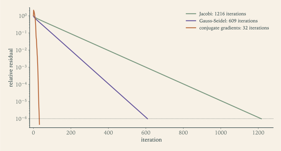
Figure 8.1 shows the qualitative difference. A stationary method does the same thing at every step. A Krylov method remembers, through its conjugate directions, everything it has already accomplished. Its residual even rises at first: conjugate gradients minimizes the energy norm of the error, which decreases at every step, and the residual norm is not obliged to follow monotonically.
Two extensions complete the picture, in outline only. Convergence depends on \(\kappa\) , so one replaces \(Ax=b\) by an equivalent system with a better-conditioned matrix, \(M^{-1}Ax=M^{-1}b\) , where the preconditioner \(M\) approximates \(A\) and is cheap to solve with; choosing \(M\) is where knowledge of the application enters. And for matrices that are not symmetric positive definite, conjugate gradients does not apply; the standard Krylov method there is GMRES, which minimizes the residual over the same Krylov subspace at the price of storing a basis for it.
The model problem of this chapter did not come from nowhere. Its matrix is what a differential equation becomes when derivatives are replaced by differences, and the last two chapters turn to differential equations: first those in which everything is known at an initial time, then those with conditions at two ends, where the linear systems of Chapters 7 and 8 reappear.
Exercises
-
Carry out two steps of power iteration, without normalization, for the matrix with rows \((2,1)\) and \((1,2)\) from \(x_0=(1,0)\) ; compute the Rayleigh quotients of \(x_1\) and \(x_2\) , and compare the reduction of their errors with the prediction of Theorem 8.1.
Solution
Multiplying, \(x_1=Ax_0=(2,1)\) and \(x_2=Ax_1=(5,4)\) ; one more product gives \(Ax_2=(14,13)\) . The Rayleigh quotients are
\[ R(x_1)=\frac{(2,1)\cdot(5,4)}{(2,1)\cdot(2,1)}=\tfrac{14}{5}=2.8,\qquad R(x_2)=\frac{(5,4)\cdot(14,13)}{(5,4)\cdot(5,4)}=\tfrac{122}{41}=2.9756 . \]The eigenvalues of \(A\) are \(3\) , with eigenvector \((1,1)\) , and \(1\) , with eigenvector \((1,-1)\) . The errors of the two Rayleigh quotients are \(0.2\) and \(0.0244\) , and their ratio is \(0.122\) .
Theorem 8.1 predicts, for this symmetric matrix, that the eigenvalue error falls by \((\lambda_2/\lambda_1)^2=\tfrac19=0.111\) per step, and that the direction error falls by \(\tfrac13\) . Both are visible. The iterates \((1,0)\) , \((2,1)\) , \((5,4)\) have components along \((1,-1)\) of relative size \(1\) , \(\tfrac13\) , \(\tfrac19\) , since \(x_k=\tfrac12\bigl(3^{k}(1,1)+(1,-1)\bigr)\) . The observed eigenvalue ratio \(0.122\) is close to \(\tfrac19\) and approaches it as \(k\) grows.
-
A symmetric matrix has eigenvalues \(10\) , \(9\) , and \(1\) . Give the convergence ratio of power iteration, the number of iterations per decimal digit of the eigenvector, and the shift \(\mu\) for which power iteration applied to \(A-\mu I\) converges fastest to the eigenvector of \(10\) , with the resulting ratio.
Answer
The ratio is \(9/10=0.9\) , so one digit takes \(1/\log_{10}(10/9)=21.9\) iterations. For \(A-\mu I\) the eigenvalues are \(10-\mu\) , \(9-\mu\) , \(1-\mu\) , and the ratio \(\max(\lvert9-\mu\rvert,\lvert1-\mu\rvert)/\lvert10-\mu\rvert\) is smallest when \(\lvert9-\mu\rvert=\lvert1-\mu\rvert\) , that is, \(\mu=5\) : the ratio is \(4/5=0.8\) , or \(10.3\) iterations per digit.
-
For a fixed nonzero vector \(x\) , show that the number \(\mu\) minimizing \(\lVert Ax-\mu x\rVert_2\) is the Rayleigh quotient \(R(x)\) , by viewing the minimization as a least-squares problem with one unknown and applying Theorem 5.7.
Solution
Minimizing \(\lVert Ax-\mu x\rVert_2\) over the single real unknown \(\mu\) is a least-squares problem in the sense of Definition 5.6: the “matrix” is the \(n\times1\) column \(x\) , the unknown is \(\mu\) , and the right-hand side is the vector \(Ax\) . Since \(x\ne0\) its one column is linearly independent, so by Theorem 5.7 the minimizer is unique and satisfies the normal equation
\[ x^{\top}x\,\mu=x^{\top}(Ax),\qquad\text{that is,}\qquad\mu=\frac{x^{\top}Ax}{x^{\top}x}=R(x). \]Equivalently, the residual \(Ax-R(x)x\) is orthogonal to \(x\) : the Rayleigh quotient is the multiple of \(x\) that best approximates \(Ax\) . This is why \(R(x)\) is the natural eigenvalue estimate to pair with an approximate eigenvector, and, combined with Theorem 8.2, it says that among all numbers \(\mu\) the Rayleigh quotient gives the tightest residual bound on the distance to an eigenvalue of a symmetric matrix.
-
Perform one step of inverse iteration with shift \(\mu=0.8\) for the matrix with rows \((2,1)\) and \((1,2)\) from \(x_0=(1,0)\) , compute the Rayleigh quotient of the result, and compare the predicted convergence ratio with that of unshifted power iteration.
Answer
\(A-0.8I\) has rows \((1.2,1)\) and \((1,1.2)\) and determinant \(0.44\) ; solving with right-hand side \((1,0)\) gives \(y=(1.2,-1)/0.44\) , a multiple of \((1.2,-1)\) . Then \(A(1.2,-1)=(1.4,-0.8)\) and \(R=(1.68+0.8)/2.44=1.0164\) , already close to the eigenvalue \(1\) . The predicted ratio is \(\lvert1-0.8\rvert/\lvert3-0.8\rvert=0.091\) per step, against \(\tfrac13\) for power iteration, which converges to the other eigenvalue.
-
Power iteration applied to the matrix with rows \((0,1)\) and \((1,0)\) from \(x_0=(1,0)\) never settles. Explain which hypothesis of Theorem 8.1 fails and show that power iteration applied to \(A+I\) converges, stating what it converges to and at what rate.
Answer
The eigenvalues are \(1\) and \(-1\) , of equal magnitude, so the hypothesis \(\lvert\lambda_1\rvert>\lvert\lambda_2\rvert\) fails; the iterates alternate between \((1,0)\) and \((0,1)\) . The matrix \(A+I\) has eigenvalues \(2\) and \(0\) with the same eigenvectors, the ratio is \(0\) , and one step gives \((1,1)\) , the eigenvector of \(A\) for the eigenvalue \(1\) .
-
For the matrix \(A\) of Example 8.1 and the unit vector \(x=(1,1,1)/\sqrt3\) , compute \(\mu=R(x)\) and \(\lVert Ax-\mu x\rVert_2\) exactly, state what Theorem 8.2 guarantees, and compare with the true eigenvalues.
Solution
With \(x=(1,1,1)/\sqrt3\) we have \(Ax=(5,5,3)/\sqrt3\) , so \(\mu=x^{\top}Ax=\tfrac{13}3\) . The residual is
\[ Ax-\mu x=\tfrac{1}{\sqrt3}\bigl(5-\tfrac{13}3,\ 5-\tfrac{13}3,\ 3-\tfrac{13}3\bigr)=\tfrac{1}{\sqrt3}\bigl(\tfrac23,\tfrac23,-\tfrac43\bigr), \]with norm \(\tfrac1{\sqrt3}\sqrt{\tfrac49+\tfrac49+\tfrac{16}9}=\sqrt{\tfrac{8}{9}}=\tfrac{2\sqrt2}{3}=0.943\) .
Theorem 8.2 guarantees an eigenvalue of \(A\) in the interval \([\mu-0.943,\mu+0.943]=[3.390,\,5.276]\) . The eigenvalues are \(1.268\) , \(3\) , and \(4.732\) . Exactly one of them, \(4.732\) , lies in the interval, at distance \(0.399\) from \(\mu\) ; the eigenvalue \(3\) lies just outside, at distance \(1.333\) . The bound is valid and, for this crude vector, loose by a factor of about \(2.4\) . As the vector improves the Rayleigh quotient error shrinks like the square of the residual, as in Theorem 8.1, so the residual bound becomes increasingly pessimistic; it remains the bound one can compute without knowing the eigenvalues.
-
The matrix with rows \((0,1)\) and \((\epsilon,0)\) has a double eigenvalue \(0\) when \(\epsilon=0\) . Find its eigenvalues for \(\epsilon=10^{-10}\) and the factor by which the perturbation has been amplified, and explain why Theorem 8.2 is not contradicted.
Answer
The characteristic equation is \(\lambda^2=\epsilon\) , so the eigenvalues are \(\pm\sqrt\epsilon=\pm10^{-5}\) : a perturbation of size \(10^{-10}\) moved them by \(10^{-5}\) , an amplification of \(10^{5}\) . The matrix is not symmetric, so Theorem 8.2 does not apply; for \(\epsilon=0\) it has only one eigenvector direction, the extreme case of nearly parallel eigenvectors.
-
Perform one step of the QR algorithm on the matrix with rows \((2,1)\) and \((1,2)\) , using Gram–Schmidt for the factorization, and verify that the result is symmetric, has the same trace and determinant, and has a smaller off-diagonal entry.
Solution
Factor. The columns are \(a_1=(2,1)\) and \(a_2=(1,2)\) . Gram–Schmidt gives \(r_{11}=\sqrt5\) and \(q_1=(2,1)/\sqrt5\) ; then \(r_{12}=q_1^{\top}a_2=4/\sqrt5\) and \(v_2=a_2-r_{12}q_1=(1,2)-\tfrac45(2,1)=(-\tfrac35,\tfrac65)\) , so \(r_{22}=\lVert v_2\rVert_2=3/\sqrt5\) and \(q_2=(-1,2)/\sqrt5\) . Thus
\[ Q=\frac1{\sqrt5}\begin{pmatrix}2&-1\\1&2\end{pmatrix},\qquad R=\frac{1}{\sqrt5}\begin{pmatrix}5&4\\0&3\end{pmatrix}. \]Recombine.
\[ A_1=RQ=\frac15\begin{pmatrix}5&4\\0&3\end{pmatrix}\begin{pmatrix}2&-1\\1&2\end{pmatrix}=\frac15\begin{pmatrix}14&3\\3&6\end{pmatrix}=\begin{pmatrix}2.8&0.6\\0.6&1.2\end{pmatrix}. \]The result is symmetric. Its trace is \(2.8+1.2=4\) and its determinant is \(3.36-0.36=3\) , the same as for \(A\) , as they must be for similar matrices; the eigenvalues are still \(3\) and \(1\) . The off-diagonal entry has fallen from \(1\) to \(0.6\) , and the diagonal entries \(2.8\) and \(1.2\) have moved toward the eigenvalues. Further steps multiply the off-diagonal entry by about \(\lambda_2/\lambda_1=\tfrac13\) each time.
-
For the system with matrix rows \((4,1)\) and \((1,3)\) and right-hand side \((1,2)\) , carry out two Jacobi sweeps and two Gauss–Seidel sweeps from the zero vector in exact fractions, and compute the spectral radius of each iteration matrix.
Solution
The exact solution is \(x=(\tfrac1{11},\tfrac7{11})=(0.0909,0.6364)\) .
Jacobi. Each sweep computes \(x_1=(1-x_2)/4\) and \(x_2=(2-x_1)/3\) from the old values. From \((0,0)\) : the first sweep gives \((\tfrac14,\tfrac23)\) , and the second gives \(\bigl((1-\tfrac23)/4,\,(2-\tfrac14)/3\bigr)\) , which is \((\tfrac1{12},\tfrac7{12})\) .
Gauss–Seidel. The new \(x_1\) is used at once. First sweep: \(x_1=\tfrac14\) , then \(x_2=(2-\tfrac14)/3=\tfrac7{12}\) . Second sweep: \(x_1=(1-\tfrac7{12})/4=\tfrac5{48}\) , then \(x_2=(2-\tfrac5{48})/3=\tfrac{91}{144}\) , giving \((\tfrac5{48},\tfrac{91}{144})=(0.1042,0.6319)\) .
Spectral radii. \(G_J\) has rows \((0,-\tfrac14)\) and \((-\tfrac13,0)\) , so its eigenvalues satisfy \(\lambda^2=\tfrac1{12}\) and \(\rho(G_J)=\sqrt{1/12}=0.289\) . For Gauss–Seidel, \(G_{GS}=-(D+L)^{-1}U\) has rows \((0,-\tfrac14)\) and \((0,\tfrac1{12})\) , with eigenvalues \(0\) and \(\tfrac1{12}\) , so \(\rho(G_{GS})=\tfrac1{12}=0.0833=\rho(G_J)^2\) . After two sweeps the largest component error is \(\tfrac7{11}-\tfrac7{12}=0.053\) for Jacobi and \(\tfrac5{48}-\tfrac1{11}=0.013\) for Gauss–Seidel; from then on Gauss–Seidel gains a factor of \(12\) per sweep and Jacobi a factor of \(12\) per two sweeps.
-
Show that the Jacobi iteration diverges for the matrix with rows \((1,2)\) and \((3,1)\) and converges after the two equations are interchanged, giving both spectral radii.
Answer
For rows \((1,2)\) and \((3,1)\) , \(G_J\) has rows \((0,-2)\) and \((-3,0)\) , eigenvalues \(\pm\sqrt6\) , and \(\rho=2.449>1\) : divergence. After the interchange the rows are \((3,1)\) and \((1,2)\) , a strictly diagonally dominant matrix; \(G_J\) has rows \((0,-\tfrac13)\) and \((-\tfrac12,0)\) and \(\rho=\sqrt{1/6}=0.408\) : convergence. The order of the equations matters to a stationary iteration.
-
Prove the Gauss–Seidel half of Theorem 8.4: if \(A\) is strictly diagonally dominant, every eigenvalue \(\lambda\) of \(G_{GS}=-(D+L)^{-1}U\) satisfies \(\lvert\lambda\rvert<1\) .
Solution
Let \(\lambda\) be an eigenvalue of \(G_{GS}\) with eigenvector \(z\ne0\) . From \(-(D+L)^{-1}Uz=\lambda z\) we get \(-Uz=\lambda(D+L)z\) , which in components reads, for every row \(i\) ,
\[ -\sum_{j>i}a_{ij}z_j=\lambda\Bigl(a_{ii}z_i+\sum_{j<i}a_{ij}z_j\Bigr). \]Scale \(z\) so that \(\max_j\lvert z_j\rvert=1\) and pick a row \(k\) with \(\lvert z_k\rvert=1\) . Taking absolute values in row \(k\) and using \(\lvert z_j\rvert\le1\) ,
\[ \lvert\lambda\rvert\Bigl(\lvert a_{kk}\rvert-\sum_{j<k}\lvert a_{kj}\rvert\Bigr)\le\lvert\lambda\rvert\,\Bigl\lvert a_{kk}z_k+\sum_{j<k}a_{kj}z_j\Bigr\rvert=\Bigl\lvert\sum_{j>k}a_{kj}z_j\Bigr\rvert\le\sum_{j>k}\lvert a_{kj}\rvert . \]Strict diagonal dominance in row \(k\) says \(\lvert a_{kk}\rvert-\sum_{j<k}\lvert a_{kj}\rvert>\sum_{j>k}\lvert a_{kj}\rvert\ge0\) , so the bracket on the left is positive and
\[ \lvert\lambda\rvert\le\frac{\sum_{j>k}\lvert a_{kj}\rvert}{\lvert a_{kk}\rvert-\sum_{j<k}\lvert a_{kj}\rvert}<1 . \]Every eigenvalue of \(G_{GS}\) has magnitude below \(1\) , so \(\rho(G_{GS})<1\) , and Theorem 8.3 gives convergence for every starting vector.
-
For the model matrix \(T_n\) with \(n=1000\) , estimate \(\rho(G_J)\) , the number of Jacobi sweeps needed to reduce the error by \(10^{-6}\) , the condition number, and the number of conjugate gradient iterations guaranteed by the bound of Section 8.6 to reduce the energy-norm error by \(10^{-6}\) .
Answer
\(\rho(G_J)=\cos(\pi/1001)\approx1-4.93\times10^{-6}\) , so about \(\ln10^{6}/(4.93\times10^{-6})=2.8\times10^{6}\) sweeps. The condition number is about \(4\cdot1001^2/\pi^2=4.06\times10^{5}\) , with square root \(637\) . The conjugate gradient bound requires \(2\bigl((\sqrt\kappa-1)/(\sqrt\kappa+1)\bigr)^{k}\le10^{-6}\) , that is, \(k\ge\tfrac12\sqrt\kappa\,\ln(2\times10^{6})\approx4600\) iterations; in exact arithmetic the method would in any case terminate within \(n=1000\) steps.
-
Carry out the conjugate gradient method by hand for the system with matrix rows \((3,1)\) and \((1,2)\) and right-hand side \((5,5)\) from \(x_0=0\) , in exact fractions, and verify that the two search directions are \(A\) -conjugate.
Solution
Start with \(x_0=0\) , so \(r_0=p_0=(5,5)\) and \(r_0^{\top}r_0=50\) . Then \(Ap_0=(20,15)\) , \(p_0^{\top}Ap_0=175\) , and
\[ \alpha_0=\tfrac{50}{175}=\tfrac27,\qquad x_1=\bigl(\tfrac{10}7,\tfrac{10}7\bigr),\qquad r_1=(5,5)-\tfrac27(20,15)=\bigl(-\tfrac57,\tfrac57\bigr). \]Next \(r_1^{\top}r_1=\tfrac{50}{49}\) , so \(\beta_0=\tfrac{50/49}{50}=\tfrac1{49}\) and
\[ p_1=r_1+\tfrac1{49}p_0=\bigl(-\tfrac{30}{49},\tfrac{40}{49}\bigr). \]Conjugacy. \(p_1^{\top}Ap_0=-\tfrac{30}{49}\cdot20+\tfrac{40}{49}\cdot15=0\) . Also \(r_1^{\top}r_0=0\) : the residuals are orthogonal.
Second step. \(Ap_1=\bigl(-\tfrac{50}{49},\tfrac{50}{49}\bigr)\) and \(p_1^{\top}Ap_1=\tfrac{1500+2000}{2401}=\tfrac{3500}{2401}\) , so
\[ \alpha_1=\tfrac{50/49}{3500/2401}=\tfrac7{10},\qquad x_2=x_1+\tfrac7{10}p_1=\bigl(\tfrac{10}7-\tfrac37,\ \tfrac{10}7+\tfrac47\bigr), \]that is, \(x_2=(1,2)\) . Check: \(A(1,2)=(3+2,\,1+4)=(5,5)\) . The method has terminated in \(n=2\) steps, as Theorem 8.6 guarantees.
Notice how little the second direction differs from the second residual: \(p_1\) is \(r_1\) plus only one forty-ninth of \(p_0\) . That small correction is the whole difference between conjugate gradients and steepest descent, which would have used \(r_1\) itself as the direction and, having started with the same first step, would then have needed infinitely many steps. The correction makes \(p_1\) conjugate to \(p_0\) , so the second line search cannot spoil the minimization already achieved along \(p_0\) .
-
Prove that nonzero vectors \(p_0,\dots,p_{m}\) that are \(A\) -conjugate with respect to a symmetric positive definite matrix \(A\) are linearly independent.
Solution
Suppose \(\sum_{i=0}^{m}c_ip_i=0\) for some scalars \(c_i\) . Fix an index \(j\) and take the inner product of both sides with \(Ap_j\) :
\[ 0=p_j^{\top}A\sum_ic_ip_i=\sum_ic_i\,p_j^{\top}Ap_i=c_j\,p_j^{\top}Ap_j , \]because every term with \(i\ne j\) vanishes by conjugacy. Since \(A\) is positive definite and \(p_j\ne0\) , the number \(p_j^{\top}Ap_j\) is strictly positive, so \(c_j=0\) . This holds for every \(j\) , so the only linear combination of the \(p_i\) that vanishes is the trivial one, and the vectors are linearly independent.
Two consequences are used in Section 8.6. There can be at most \(n\) conjugate directions in \(\mathbb R^{n}\) , and any \(n\) of them form a basis, which is why minimizing over their span is minimizing over the whole space. The argument is the same as the proof that orthogonal vectors are independent; conjugacy is orthogonality in the inner product \(\langle u,v\rangle=u^{\top}Av\) , and positive definiteness is what makes that an inner product.
-
For a symmetric positive definite matrix with \(\kappa_2=100\) , compare the number of steepest-descent iterations and of conjugate gradient iterations needed to guarantee a reduction of the energy-norm error by \(10^{-6}\) , using the ratio \((\kappa-1)/(\kappa+1)\) and the bound of Section 8.6.
Answer
Steepest descent: \((99/101)^{k}\le10^{-6}\) requires \(k\ge\ln10^{6}/\ln(101/99)=691\) . Conjugate gradients: \(2(9/11)^{k}\le10^{-6}\) requires \(k\ge\ln(2\times10^{6})/\ln(11/9)=72.3\) , so \(73\) . The dependence on \(\sqrt\kappa\) instead of \(\kappa\) is worth a factor of nearly ten here and grows with \(\kappa\) .
-
The conjugate gradient listing is applied to the symmetric but indefinite diagonal matrix with entries \(1\) and \(-1\) and right-hand side \((1,1)\) from \(x_0=0\) . Show what happens in the first step and explain which property of positive definite matrices the method relies on.
Answer
\(r_0=p_0=(1,1)\) , \(Ap_0=(1,-1)\) , and \(p_0^{\top}Ap_0=1-1=0\) : the step length \(\alpha_0=rr/(p^{\top}Ap)\) divides by zero. The method relies on \(p^{\top}Ap>0\) for every nonzero \(p\) , which is positive definiteness; it is what makes \(\phi\) have a minimum along every line and makes \(\lVert\cdot\rVert_A\) a norm.
-
An iterative solver stops when the relative residual is below \(10^{-8}\) , for a matrix with \(\kappa_2=10^{6}\) . Use Corollary 7.7 to state what is guaranteed about the relative error, and give a stopping tolerance that guarantees six correct digits.
Answer
By Corollary 7.7 the relative error is at most \(\kappa\times10^{-8}=10^{-2}\) : only two digits are guaranteed. For six digits the relative residual must be at most \(10^{-6}/\kappa=10^{-12}\) .
-
For the system of Example 8.5, regard the Jacobi iteration as a fixed-point iteration, show that it is a contraction in the \(\infty\) -norm with constant \(L=\tfrac12\) , and use the a posteriori bound of Theorem 3.2, with norms in place of absolute values, to bound the error of the eighth iterate from the seventh and eighth iterates; compare with the true error.
Solution
The Jacobi iteration is \(x^{(k+1)}=g(x^{(k)})\) with \(g(x)=G_Jx+c\) . For any two vectors, \(\lVert g(x)-g(y)\rVert_\infty=\lVert G_J(x-y)\rVert_\infty\le\lVert G_J\rVert_\infty\lVert x-y\rVert_\infty\) , and for the matrix of Example 8.5 the rows of \(G_J\) are \((0,\tfrac14,0)\) , \((\tfrac14,0,\tfrac14)\) , \((0,\tfrac14,0)\) , with largest absolute row sum \(\tfrac12\) . So \(g\) is a contraction on \(\mathbb R^3\) in the \(\infty\) -norm with \(L=\tfrac12\) .
The proof of the a posteriori bound in Theorem 3.2 used only the triangle inequality and the contraction property, so it holds with norms: \(\lVert x^{(k)}-x\rVert_\infty\le\tfrac{L}{1-L}\lVert x^{(k)}-x^{(k-1)}\rVert_\infty\) . The seventh and eighth iterates are \((0.99902,1.99805,2.99902)\) and \((0.99951,1.99951,2.99951)\) , which differ by at most \(0.00146\) , in the middle component. With \(L/(1-L)=1\) the bound is \(0.00146\) . The true error of the eighth iterate is \(0.00049\) . The bound holds and overestimates by a factor of three, because \(L=\tfrac12\) is the norm of \(G_J\) while the error actually contracts at the rate \(\rho(G_J)=0.354\) ; with \(\rho\) in place of \(L\) the estimate \(\tfrac{\rho}{1-\rho}\times0.00146=0.00080\) is closer.
-
Verify that the vector \(v\) with components \(v_i=\sin\bigl(ij\pi/(n+1)\bigr)\) , \(i=1,\dots,n\) , is an eigenvector of the model matrix \(T_n\) with eigenvalue \(2-2\cos\bigl(j\pi/(n+1)\bigr)\) , for each \(j=1,\dots,n\) .
Solution
Let \(\theta=j\pi/(n+1)\) , so \(v_i=\sin(i\theta)\) . The formula also gives \(v_0=\sin0=0\) and \(v_{n+1}=\sin(j\pi)=0\) , so for every \(i=1,\dots,n\) , including the first and last rows where one neighbour is absent, the \(i\) -th component of \(T_nv\) can be written
\[ (T_nv)_i=-v_{i-1}+2v_i-v_{i+1}=2\sin(i\theta)-\bigl(\sin((i-1)\theta)+\sin((i+1)\theta)\bigr). \]The identity \(\sin(\alpha-\beta)+\sin(\alpha+\beta)=2\sin\alpha\cos\beta\) with \(\alpha=i\theta\) and \(\beta=\theta\) gives \(\sin((i-1)\theta)+\sin((i+1)\theta)=2\sin(i\theta)\cos\theta\) . Hence
\[ (T_nv)_i=(2-2\cos\theta)\sin(i\theta)=(2-2\cos\theta)\,v_i . \]The vector \(v\) is not zero, since \(v_1=\sin\theta>0\) for \(0<\theta<\pi\) . So \(v\) is an eigenvector with eigenvalue \(2-2\cos\bigl(j\pi/(n+1)\bigr)\) . The \(n\) values of \(j\) give \(n\) distinct eigenvalues, because the cosine is strictly decreasing on \((0,\pi)\) , so these are all the eigenvalues of \(T_n\) . The smallest is \(2-2\cos\bigl(\pi/(n+1)\bigr)\approx\pi^2/(n+1)^2\) and the largest is close to \(4\) , which gives the condition number quoted in Section 8.5, and \(G_J=I-\tfrac12T_n\) has eigenvalues \(\cos\bigl(j\pi/(n+1)\bigr)\) .
-
A symmetric positive definite matrix has diagonal entries ranging from \(1\) to \(10^{6}\) and small off-diagonal entries. Explain why conjugate gradients converges slowly on it, and how the diagonal preconditioner \(M=D\) changes the matrix whose condition number governs the convergence.
Hint
Use Exercise 7.14 to see that the extreme eigenvalues of \(A\) are of the order of its smallest and largest diagonal entries, so \(\kappa_2(A)\) is about \(10^{6}\) . Then consider the symmetrically scaled matrix \(D^{-1/2}AD^{-1/2}\) : what is its diagonal, and how large are its off-diagonal entries?