The equation \(y'=-50\,(y-\cos t)\) with \(y(0)=0\) describes a quantity that is pulled toward the slowly varying target \(\cos t\) at a rate of \(50\) per unit time. Its solution rushes from \(0\) up to the target in about a tenth of a time unit and then follows it closely; at \(t=1\) it is \(0.5569\) . Compute it with the simplest numerical method, Euler’s, and a step \(h=0.05\) . Twenty steps give \(y(1)\approx-3325\) . The step was not too coarse to describe the solution, which after the first moments is as smooth as a cosine. Reduce the step to \(h=0.03\) and the same method gives an error of \(2\times10^{-4}\) .
Between those two steps lies a threshold that has nothing to do with accuracy. This chapter develops numerical methods for initial-value problems along two separate lines that the example forces apart. The first is convergence: how the error behaves as \(h\to0\) , what order a method has, how to get high order cheaply. The second is stability: how a method behaves at the finite step actually used, and why some problems, called stiff, impose a severe step restriction on explicit methods that no amount of order can lift. A third theme connects them in practice, the automatic choice of the step from an estimate of the local error.
9.1 Euler’s method and the meaning of convergence
The problem is to find \(y\) on \([t_0,T]\) with
We assume throughout that \(f\)
is continuous and satisfies a Lipschitz condition in its second argument: \(\lvert f(t,y)-f(t,z)\rvert\le L\lvert y-z\rvert\)
for all \(t\)
in the interval and all \(y,z\)
. Under these hypotheses the problem has exactly one solution, by the Picard–Lindelöf theorem of Differential Equations (math.differential-equations.picard-lindelof). A numerical method produces values \(y_n\approx y(t_n)\)
on a grid \(t_n=t_0+nh\)
.
Euler’s method follows the tangent line for one step:
Example 9.1: Four Euler steps
For \(y'=-2ty\) , \(y(0)=1\) , the solution is \(y(t)=e^{-t^2}\) . With \(h=0.25\) :
The exact value is \(y(1)=e^{-1}=0.367879\) , so the error is \(0.0423\) . Each step uses the slope at the left end of its interval, and since the solution is curving downward faster and faster on \([0,0.7]\) the method lags above it.
How does this error depend on \(h\) ? The analysis separates what happens in one step from how the effects of many steps combine.
Definition 9.1 (one-step method, local truncation error, order). A one-step method has the form \(y_{n+1}=y_n+h\,\Phi(t_n,y_n,h)\) . Its local truncation error at \(t_{n+1}\) is the amount by which the exact solution fails to satisfy the scheme, per unit step:
The method is consistent of order \(p\) if \(\lvert\tau_n\rvert\le Ch^{p}\) for smooth solutions.
For Euler’s method \(\Phi=f\) , and Taylor’s theorem gives \(y(t_{n+1})=y(t_n)+hy'(t_n)+\tfrac12h^2y''(\xi)\) with \(y'(t_n)=f(t_n,y(t_n))\) , so \(\tau_{n+1}=\tfrac12h\,y''(\xi)\) : Euler’s method is consistent of order \(1\) .
9.2 From local error to global error
A local error is committed at every step, and each one is then carried forward by the method. The next theorem shows that the carried errors do not pile up worse than the Lipschitz constant allows.
Theorem 9.2 (convergence of one-step methods). Suppose \(\Phi\) satisfies \(\lvert\Phi(t,y,h)-\Phi(t,z,h)\rvert\le\Lambda\lvert y-z\rvert\) and the local truncation errors satisfy \(\lvert\tau_n\rvert\le\tau\) for all \(n\) . Then with \(y_0=y(t_0)\) ,
In particular a method consistent of order \(p\) has global error \(O(h^{p})\) on a fixed interval. For Euler’s method, with \(\lvert y''\rvert\le M\) , the bound is \(\dfrac{hM}{2L}\bigl(e^{L(t_n-t_0)}-1\bigr)\) .
Proof. Let \(e_n=y(t_n)-y_n\) . By the definition of \(\tau_{n+1}\) , \(y(t_{n+1})=y(t_n)+h\Phi(t_n,y(t_n),h)+h\tau_{n+1}\) . Subtracting the scheme,
With \(e_0=0\) , induction gives \(\lvert e_n\rvert\le h\tau\sum_{j=0}^{n-1}(1+h\Lambda)^{j}=\tau\bigl((1+h\Lambda)^{n}-1\bigr)/\Lambda\) , and \((1+h\Lambda)^{n}\le e^{nh\Lambda}=e^{\Lambda(t_n-t_0)}\) .
The structure of the proof is the structure of the subject. Consistency controls the error injected per step. A stability property, here the Lipschitz bound that keeps the method from amplifying errors by more than \(1+h\Lambda\) per step, controls how injected errors propagate. Together they give convergence. A local error of size \(h\tau=O(h^{p+1})\) is committed at each of \(O(1/h)\) steps, and the global error is \(O(h^{p})\) .
Rounding enters the same recursion as an extra error \(\delta\) per step, which adds \(\delta/h\) to \(\tau\) . The total bound then has the form \(C(hM/2+\delta/h)\) , the same competition as in Theorem 1.11. In double precision the minimizing step is near \(10^{-8}\) and is never approached in practice; in single precision it is near \(3\times10^{-4}\) and limits Euler’s method to about three digits.
Example 9.2: First-order convergence, observed and bounded
Continue Example 9.1 with \(n\) steps on \([0,1]\) . The errors \(y_n-y(1)\) are:
| \(n\) | \(4\) | \(8\) | \(16\) | \(32\) | \(64\) |
|---|---|---|---|---|---|
| error | \(4.228\times10^{-2}\) | \(1.784\times10^{-2}\) | \(8.254\times10^{-3}\) | \(3.975\times10^{-3}\) | \(1.951\times10^{-3}\) |
| observed order | \(1.25\) | \(1.11\) | \(1.05\) | \(1.03\) |
The order settles toward \(1\) : halving the step halves the error. For the bound, \(\lvert\partial f/\partial y\rvert=2t\le2\) gives \(L=2\) , and \(y''=(4t^2-2)e^{-t^2}\) gives \(M=2\) , so Theorem 9.2 yields \(\lvert e_n\rvert\le\tfrac{2h}{4}(e^{2}-1)=3.19\,h\) . The observed errors are about \(0.125\,h\) . The bound is correct and twenty-five times too large, because it assumes that every local error is of maximal size and is amplified at the maximal rate \(e^{L(T-t)}\) , while for this equation, whose solutions converge toward one another, errors are in fact damped. Convergence bounds of this kind establish the order. They are rarely useful as estimates of the error.
9.3 Runge–Kutta methods
First order is too slow. Six digits from Euler’s method on the example would take about \(123\,000\) steps. Higher order can be had by matching more terms of the Taylor expansion of the solution, and the Runge–Kutta idea is to do so without differentiating \(f\) , by evaluating \(f\) at several points within the step.
The midpoint method takes an Euler half-step to estimate the slope in the middle of the interval and uses that slope for the whole step:
Heun’s method averages the slopes at the two ends, the second computed from an Euler prediction:
Both are of order \(2\) . To see why for the midpoint method, expand \(k_2\) about \((t_n,y_n)\) along the exact solution: \(k_2=f+\tfrac12h(f_t+f_yf)+O(h^2)\) , where \(f_t+f_yf=y''\) by the chain rule. So \(y_n+hk_2=y_n+hy'+\tfrac12h^2y''+O(h^3)\) , which agrees with the Taylor expansion of \(y(t_{n+1})\) through the term in \(h^2\) ; the local truncation error is \(O(h^2)\) .
The classical fourth-order Runge–Kutta method uses four evaluations:
Its local truncation error is \(O(h^4)\) ; the verification is a longer Taylor expansion of the same kind and we omit it. When \(f\) does not depend on \(y\) the method reduces to Simpson’s rule (Exercise 9.17), which makes the weights \(\tfrac16,\tfrac26,\tfrac26,\tfrac16\) less mysterious. Each of these methods has an increment function \(\Phi\) that inherits a Lipschitz condition from \(f\) , so Theorem 9.2 applies and the global orders are \(2\) , \(2\) , and \(4\) .
Example 9.3: Order and cost compared
On the problem of Example 9.1 the errors at \(t=1\) are:
| \(n\) | Euler | midpoint | order | fourth-order | order |
|---|---|---|---|---|---|
| \(4\) | \(4.228\times10^{-2}\) | \(-6.028\times10^{-3}\) | \(5.505\times10^{-5}\) | ||
| \(8\) | \(1.784\times10^{-2}\) | \(-1.188\times10^{-3}\) | \(2.34\) | \(3.927\times10^{-6}\) | \(3.81\) |
| \(16\) | \(8.254\times10^{-3}\) | \(-2.657\times10^{-4}\) | \(2.16\) | \(2.501\times10^{-7}\) | \(3.97\) |
| \(32\) | \(3.975\times10^{-3}\) | \(-6.301\times10^{-5}\) | \(2.08\) | \(1.565\times10^{-8}\) | \(4.00\) |
| \(64\) | \(1.951\times10^{-3}\) | \(-1.535\times10^{-5}\) | \(2.04\) | \(9.768\times10^{-10}\) | \(4.00\) |
The fair comparison is by work. To bring the error below \(10^{-6}\) , Euler’s method needs \(122\,628\) steps and as many evaluations of \(f\) ; the midpoint method needs \(249\) steps, \(498\) evaluations; the fourth-order method needs \(12\) steps, \(48\) evaluations. Higher order costs more per step and repays it thousands of times over when the solution is smooth and the accuracy demanded is high.
9.4 Stability on a test equation
Return to the opening experiment. Convergence theory describes the limit \(h\to0\) . To understand a fixed \(h\) , apply the method to the simplest equation with a decaying solution, the test equation
whose solutions \(e^{\lambda t}\) tend to zero. Euler’s method gives \(y_{n+1}=(1+h\lambda)y_n\) , so \(y_n=(1+h\lambda)^{n}y_0\) . The numerical solution decays if and only if \(\lvert1+h\lambda\rvert<1\) . For real \(\lambda<0\) that is the condition
If it is violated the numerical solution grows geometrically and alternates in sign, whatever the accuracy of the method.
Definition 9.3 (stability function, region of absolute stability). Applied to the test equation, a one-step method gives \(y_{n+1}=R(h\lambda)\,y_n\) for a function \(R\) called its stability function. The region of absolute stability is \(\{z\in\mathbb C:\lvert R(z)\rvert\le1\}\) . The method is A-stable if this region contains the whole left half-plane \(\operatorname{Re}z\le0\) .
For Euler’s method \(R(z)=1+z\) and the region is the disc of radius \(1\) centred at \(-1\) . For the midpoint and Heun methods \(R(z)=1+z+\tfrac12z^2\) , and for the fourth-order method \(R(z)=1+z+\tfrac12z^2+\tfrac16z^3+\tfrac1{24}z^4\) ; in each case \(R\) is the Taylor polynomial of \(e^{z}\) of degree equal to the order, as it must be, since the exact solution multiplies by \(e^{h\lambda}\) per step. On the negative real axis the stability intervals are \([-2,0]\) for the first three and \([-2.785,0]\) for the fourth-order method. At an endpoint of the interval \(\lvert R\rvert=1\) and perturbations neither grow nor decay; for them to die out \(h\lambda\) must lie strictly inside. Every explicit Runge–Kutta method has a polynomial for \(R\) , and a polynomial is unbounded as \(z\to-\infty\) , so no explicit method of this kind is A-stable.
The test equation is not a toy. For a linear system \(y'=Ay\)
with a basis of eigenvectors, the components of the solution along the eigenvectors each satisfy a test equation with \(\lambda\)
an eigenvalue of \(A\)
; this is the decoupling behind the matrix-exponential solution of Differential Equations (math.differential-equations.matrix-exponential-solution). A one-step method applied to the system is stable only if \(h\lambda\)
lies in its stability region for every eigenvalue. For a nonlinear problem the eigenvalues of the Jacobian \(\partial f/\partial y\)
along the solution play the same role locally.
Example 9.4: The threshold in the opening problem
For \(y'=-50(y-\cos t)\) the relevant \(\lambda\) is \(-50\) , and Euler’s method requires \(h<2/50=0.04\) for the transient to decay. The exact solution is \(y(t)=\bigl(2500\cos t+50\sin t-2500e^{-50t}\bigr)/2501\) .
With \(h=0.05\) , so that \(h\lambda=-2.5\) and the amplification factor is \(1+h\lambda=-1.5\) , the first Euler values are
an oscillation growing by the factor \(1.5\) per step, reaching \(-3325\) at \(t=1\) . With \(h=0.04\) , the endpoint of the stability interval, the factor is exactly \(-1\) and the values oscillate without growing or decaying. With \(h=0.03\) the factor is \(-0.5\) , the initial disturbance dies out within a few steps, and at \(t=0.99\) the computed value \(0.565356\) differs from the exact \(0.565184\) by \(1.7\times10^{-4}\) .
The fourth-order method fares slightly better and no differently in kind: it requires \(h<2.785/50=0.0557\) .
9.5 Stiffness and implicit methods
In Example 9.4 the solution after \(t=0.2\) is indistinguishable from a smooth curve that a step of \(0.2\) or more could represent to several digits. The fast transient \(e^{-50t}\) has long since vanished from the solution. It has not vanished from the differential equation, and an explicit method must go on using a step small enough to keep it from being resurrected.
A problem is called stiff when stability, not accuracy, dictates the step size of explicit methods. It happens when the problem contains time scales that differ by orders of magnitude, a fast decay rate \(\lvert\lambda\rvert\) alongside a solution that varies on a scale of order \(1\) : explicit methods then need of the order of \(\lvert\lambda\rvert T\) steps to cover an interval of length \(T\) , however smooth the solution is.
The cure is a method whose stability region contains the whole negative real axis. The backward Euler method uses the slope at the end of the step:
It is implicit: \(y_{n+1}\) appears on both sides, and each step requires solving an equation, by Newton’s method in general (Chapter 3), with a linear system to solve at each iteration when \(y\) is a vector (Chapter 7). On the test equation \(y_{n+1}=y_n+h\lambda y_{n+1}\) gives \(R(z)=1/(1-z)\) , and \(\lvert R(z)\rvert\le1\) whenever \(\operatorname{Re}z\le0\) : backward Euler is A-stable (Exercise 9.10). It is of order \(1\) , like Euler’s method. The trapezoidal method \(y_{n+1}=y_n+\tfrac12h\bigl(f(t_n,y_n)+f(t_{n+1},y_{n+1})\bigr)\) is also A-stable and has order \(2\) .
Example 9.5: Backward Euler on the stiff problem
For \(y'=-50(y-\cos t)\) the implicit equation is linear and can be solved by hand: \(y_{n+1}=\bigl(y_n+50h\cos t_{n+1}\bigr)/(1+50h)\) . With \(h=0.1\) , a step two and a half times larger than the stability limit of the explicit method:
| \(t_n\) | \(0.1\) | \(0.2\) | \(0.3\) | \(0.4\) | \(1.0\) |
|---|---|---|---|---|---|
| backward Euler | \(0.8292\) | \(0.9549\) | \(0.9553\) | \(0.9268\) | \(0.5563\) |
| exact | \(0.9899\) | \(0.9836\) | \(0.9609\) | \(0.9285\) | \(0.5569\) |
The first step, which straddles the transient, is inaccurate, as it must be with \(h=0.1\) . After that the method tracks the smooth solution, and at \(t=1\) the error is \(6.0\times10^{-4}\) with ten steps. Explicit Euler needed \(h<0.04\) merely to avoid blowing up. Each backward Euler step multiplies inherited errors by \(1/(1+50h)=\tfrac16\) , so the transient is damped more strongly, not less, as \(h\) grows.
The trapezoidal method with the same step gives \(1.4250\) , \(0.8000\) , \(1.0396\) , \(0.8948\) at the first four points and an error of \(2.0\times10^{-4}\) at \(t=1\) . It is stable, but its amplification factor \(R(-5)=(1-2.5)/(1+2.5)=-0.43\) damps the initial disturbance slowly and with alternating sign. A-stability guarantees that errors do not grow. It does not guarantee that stiff components are removed quickly.
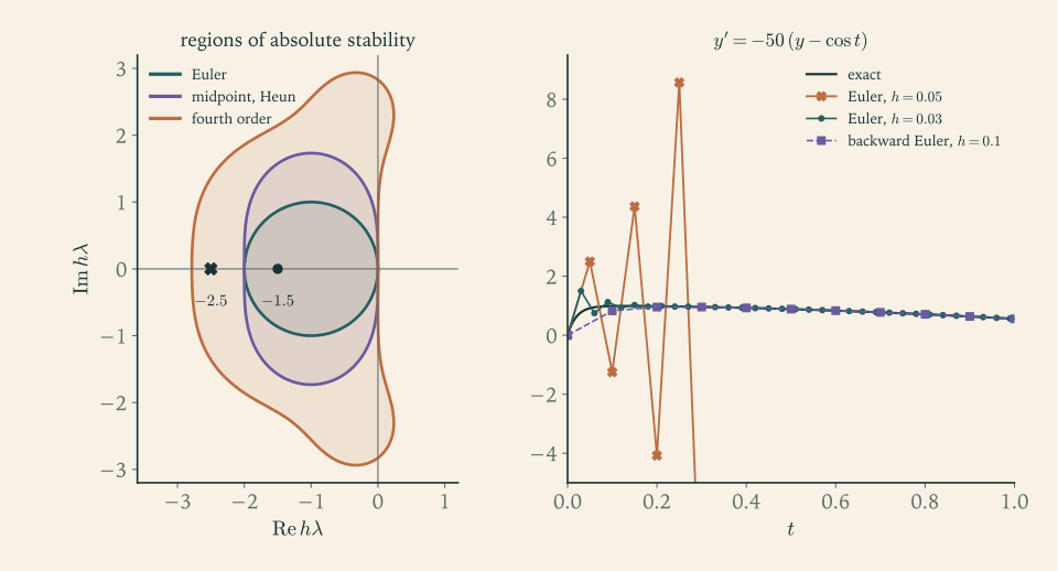
Figure 9.1 joins the two halves of the argument. The point \(h\lambda=-2.5\) lies outside the Euler disc and the computation on the right diverges; the point \(-1.5\) lies inside and the computation settles down. Raising the order enlarges the region a little. Only an implicit method removes the restriction.
Common mistake. Responding to an oscillating, growing numerical solution by switching to a higher-order explicit method, or by tightening an accuracy tolerance, without asking whether the trouble is instability. The signature of instability is growth by a roughly constant factor per step, usually with alternating sign, at a step size for which the true solution is smooth. Estimate the largest \(\lvert\lambda\rvert\) of the Jacobian and compare \(h\lvert\lambda\rvert\) with the stability interval of the method. If the stable step is far smaller than accuracy requires, the problem is stiff, and the remedy is an implicit method.
9.6 Choosing the step automatically
A fixed step is wasteful when the solution changes character, and no user knows in advance what step a given accuracy requires. Practical codes estimate the local error at every step and adjust \(h\) . The simplest device uses a pair of methods of different order that share their function evaluations. Heun’s method computes \(k_1\) and \(k_2\) , from which the Euler value \(y_n+hk_1\) is free; the difference of the two results,
estimates the local error of the lower-order one. If \(\mathrm{est}\le\mathrm{tol}\) the step is accepted, with the Heun value; otherwise it is rejected and repeated. Either way the next step is chosen so that the predicted estimate equals the tolerance, with a safety factor: since \(\mathrm{est}\) is proportional to \(h^2\) ,
For a pair in which the lower-order method has local error proportional to \(h^{q}\) , the square root becomes the power \(1/q\) . Production codes use pairs of orders four and five built on the same principle.
Example 9.6: A front, and what local error control does and does not deliver
The logistic equation \(y'=20\,y(1-y)\) with \(y(0)=10^{-4}\) has the solution \(y(t)=1/\bigl(1+9999e^{-20t}\bigr)\) : nearly zero at first, a rapid rise through \(\tfrac12\) at \(t=0.4605\) , then nearly \(1\) . Integrate to \(T=10\) with the Heun–Euler pair, tolerance \(10^{-5}\) , initial step \(0.01\) , and no step allowed to exceed five times its predecessor.
The integration takes \(683\) accepted steps and \(10\) rejected ones. Of the accepted steps, \(456\) lie in the interval \([0.3,0.7]\) around the front, where the step shrinks to \(6.5\times10^{-4}\) . Before the front the steps are larger, and after it they grow to about \(0.1\) and stay there: every accepted step that begins after \(t=2\) , apart from the shortened last one, lies between \(0.0988\) and \(0.1012\) . That plateau is not an accuracy limit, since the solution there is constant to many digits. On the upper branch \(\partial f/\partial y=20(1-2y)\approx-20\) , the stability limit of Heun’s method is \(h<2/20=0.1\) , and whenever the controller tries a larger step the incipient instability shows up in the error estimate and the step is cut back. The controller has found the stability limit by itself. The problem is mildly stiff on \([1,10]\) .
The largest global error along the trajectory is \(6.1\times10^{-3}\) , six hundred times the tolerance. The tolerance controls the error committed in each step. Before the front \(\partial f/\partial y\approx+20\) , so neighbouring solutions diverge like \(e^{20t}\) , and local errors made early are amplified by the time the front arrives. Step-size control regulates local error; the global error is whatever the differential equation makes of it. A fixed-step Heun integration needs about \(1400\) steps to match the same global accuracy, twice the adaptive count, and the advantage grows with the length of the quiet interval.
9.7 Systems
Everything in this chapter applies unchanged to systems \(y'=f(t,y)\) with \(y\in\mathbb R^{m}\) : the formulas are the same with vectors for \(y\) and the \(k_i\) , and absolute values become norms in Theorem 9.2. An equation of higher order is first rewritten as a system. For \(u''=g(t,u,u')\) , put \(y=(u,u')\) ; then \(y'=(y_2,\,g(t,y_1,y_2))\) .
Example 9.7: An oscillator, and what each method does to its energy
The equation \(u''=-u\) with \(u(0)=1\) , \(u'(0)=0\) becomes \(y'=Ay\) with \(A=\begin{pmatrix}0&1\\-1&0\end{pmatrix}\) , whose eigenvalues are \(\pm i\) . The solution \((\cos t,-\sin t)\) moves on the unit circle; the squared radius \(u^2+u'^2\) is twice the energy and is constant.
Euler’s method multiplies each eigencomponent by \(1+ih\) per step, and \(\lvert1+ih\rvert=\sqrt{1+h^2}>1\) : the purely imaginary \(h\lambda\) lies outside the stability disc for every \(h\) . With \(h=0.1\) the radius after \(100\) steps, at \(t=10\) , is \((1.01)^{50}=1.645\) . The computed point is \((-1.409,\,0.849)\) where the true one is \((-0.839,\,0.544)\) : the phase is nearly right and the amplitude is \(64\) percent too large. Backward Euler multiplies by \(1/(1-ih)\) , of magnitude \(1/\sqrt{1+h^2}\) , and the radius decays to \(0.608\) . Neither method is acceptable for a long oscillation, and for opposite reasons.
The fourth-order method has \(\lvert R(ih)\rvert=1-\tfrac1{144}h^6+\cdots\) , just below \(1\) . With \(h=0.1\) the radius after \(100\) steps is \(0.99999931\) , and the computed point differs from the true one by less than \(10^{-5}\) . Its stability region includes the segment of the imaginary axis up to \(\pm2.83\,i\) , which is what makes it suitable for oscillatory problems.
One-step methods are not the only kind. Multistep methods reuse values of \(f\) from previous steps: the two-step Adams–Bashforth method \(y_{n+1}=y_n+\tfrac12h\bigl(3f(t_n,y_n)-f(t_{n-1},y_{n-1})\bigr)\) achieves second order with one new evaluation per step. Their theory requires a stability condition of a new kind, on the roots of a polynomial associated with the method, and their implicit members, the backward differentiation formulas, are the standard tools for stiff systems. We do not pursue them.
In an initial-value problem all the data sit at one point and the solution is marched forward from it. The final chapter takes up problems in which the data are split between two ends of an interval. There is then no starting point to march from, the unknowns are coupled across the whole interval, and the linear systems of Chapters 7 and 8 return.
Exercises
-
Carry out two steps of Euler’s method with \(h=0.1\) for \(y'=t+y\) , \(y(0)=1\) , and compare the result with the exact solution \(y(t)=2e^{t}-t-1\) at \(t=0.2\) .
Answer
\(y_1=1+0.1(0+1)=1.1\) and \(y_2=1.1+0.1(0.1+1.1)=1.22\) . The exact value is \(y(0.2)=2e^{0.2}-1.2=1.242806\) , so the error is \(0.0228\) .
-
For the problem of Exercise 9.1, take one step of Heun’s method and one step of the midpoint method with \(h=0.2\) , and compare the errors at \(t=0.2\) with that of the two Euler steps.
Answer
Heun: \(k_1=f(0,1)=1\) , \(k_2=f(0.2,1.2)=1.4\) , \(y_1=1+0.1(1+1.4)=1.24\) . Midpoint: \(k_1=1\) , \(k_2=f(0.1,1.1)=1.2\) , \(y_1=1+0.2(1.2)=1.24\) . Both have error \(0.0028\) , eight times smaller than the two Euler steps, for the same two evaluations of \(f\) .
-
Apply one step of the classical fourth-order Runge–Kutta method to \(y'=y\) , \(y(0)=1\) , with \(h=0.1\) , listing \(k_1\) to \(k_4\) , and show that for \(y'=\lambda y\) the method gives \(y_{n+1}=R(h\lambda)y_n\) with \(R\) the Taylor polynomial of degree \(4\) of the exponential.
Solution
With \(f(t,y)=y\) , \(y_0=1\) , and \(h=0.1\) :
\[ k_1=1,\qquad k_2=1+0.05\,k_1=1.05,\qquad k_3=1+0.05\,k_2=1.0525,\qquad k_4=1+0.1\,k_3=1.10525 . \]Then \(y_1=1+\tfrac{0.1}{6}(1+2.1+2.105+1.10525)=1+\tfrac{0.1}{6}(6.31025)\) , that is, \(y_1=1.10517083\) . The exact value is \(e^{0.1}=1.10517092\) , so the error is \(8.5\times10^{-8}\) .
For the general test equation put \(z=h\lambda\) and \(y_n=1\) for convenience; the slopes are \(\lambda\) times
\[ s_1=1,\qquad s_2=1+\tfrac12z,\qquad s_3=1+\tfrac12z\,s_2=1+\tfrac12z+\tfrac14z^2,\qquad s_4=1+z\,s_3=1+z+\tfrac12z^2+\tfrac14z^3 . \]The update is \(y_{n+1}=1+\tfrac16z\,(s_1+2s_2+2s_3+s_4)\) . Adding, \(s_1+2s_2+2s_3+s_4=6+3z+z^2+\tfrac14z^3\) , so
\[ y_{n+1}=1+z+\tfrac12z^2+\tfrac16z^3+\tfrac1{24}z^4=R(z), \]the Taylor polynomial of degree \(4\) of \(e^{z}\) . By linearity the same factor multiplies any \(y_n\) . The numerical value above is \(R(0.1)\) , and its error is the first omitted Taylor term, \(0.1^5/120=8.3\times10^{-8}\) , to leading order.
-
Show that the local truncation error of the backward Euler method is \(-\tfrac12h\,y''(\xi)\) for some \(\xi\) in the step, and that of the trapezoidal method is \(O(h^2)\) , assuming the solution is sufficiently smooth.
Solution
For an implicit method the local truncation error is defined in the same way as in Definition 9.1: substitute the exact solution into the scheme and divide the defect by \(h\) .
Backward Euler. The defect is \(\tau_{n+1}=\bigl(y(t_{n+1})-y(t_n)\bigr)/h-f\bigl(t_{n+1},y(t_{n+1})\bigr)=\bigl(y(t_{n+1})-y(t_n)\bigr)/h-y'(t_{n+1})\) . Expand \(y(t_n)\) about \(t_{n+1}\) by Taylor’s theorem: \(y(t_n)=y(t_{n+1})-hy'(t_{n+1})+\tfrac12h^2y''(\xi)\) for some \(\xi\in(t_n,t_{n+1})\) . Substituting,
\[ \tau_{n+1}=y'(t_{n+1})-\tfrac12h\,y''(\xi)-y'(t_{n+1})=-\tfrac12h\,y''(\xi). \]This is the same size as Euler’s local truncation error, with the opposite sign: backward Euler is consistent of order \(1\) .
Trapezoidal method. The defect is \(\bigl(y(t_{n+1})-y(t_n)\bigr)/h-\tfrac12\bigl(y'(t_n)+y'(t_{n+1})\bigr)\) . With all derivatives evaluated at \(t_n\) , \(y(t_{n+1})-y(t_n)=hy'+\tfrac12h^2y''+\tfrac16h^3y'''+O(h^4)\) and \(y'(t_{n+1})=y'+hy''+\tfrac12h^2y'''+O(h^3)\) . Hence
\[ \tau_{n+1}=\bigl(y'+\tfrac12hy''+\tfrac16h^2y'''\bigr)-\bigl(y'+\tfrac12hy''+\tfrac14h^2y'''\bigr)+O(h^3)=-\tfrac1{12}h^2y'''+O(h^3), \]so the method is of order \(2\) . The constant \(\tfrac1{12}\) is that of the trapezoid quadrature rule in Theorem 6.2, as it should be.
-
Use Theorem 9.2 to bound the error of Euler’s method for \(y'=-y\) , \(y(0)=1\) , at \(t=1\) with \(h=0.1\) , compute the actual error, and explain the discrepancy.
Solution
Here \(f(t,y)=-y\) , so \(L=1\) , and the solution \(y=e^{-t}\) has \(\lvert y''\rvert=e^{-t}\le1\) on \([0,1]\) , so \(M=1\) . Theorem 9.2 gives
\[ \lvert e_n\rvert\le\frac{hM}{2L}\bigl(e^{L\cdot1}-1\bigr)=0.05\,(e-1)=0.0859 . \]Euler’s method gives \(y_{10}=(1-0.1)^{10}=0.348678\) , and \(e^{-1}=0.367879\) , so the actual error is \(0.0192\) . The bound is valid and \(4.5\) times too large.
The discrepancy has a clear source. The proof bounds the propagation of each local error by the factor \(1+hL\) per step, as if errors could grow like \(e^{Lt}\) . For this equation they shrink: an error \(e_n\) becomes \((1-h)e_n\) at the next step, because \(\partial f/\partial y=-1\) is negative. The Lipschitz constant records the size of \(\partial f/\partial y\) and discards its sign. For equations whose solutions converge toward one another the bound is therefore always pessimistic, and for long intervals wildly so, since it grows like \(e^{LT}\) while the true error stays bounded.
-
From the Euler errors for \(n=16\) and \(n=32\) in Example 9.2, compute the observed order and predict the error for \(n=1000\) ; state the assumption behind the prediction.
Answer
The observed order is \(\log_2(8.254/3.975)=1.05\) . Assuming the error is proportional to \(h\) , which the order close to \(1\) supports, the error at \(n=1000\) is about \(3.975\times10^{-3}\times32/1000=1.3\times10^{-4}\) .
-
Rewrite \(u''+4u=\sin t\) , \(u(0)=1\) , \(u'(0)=0\) , as a first-order system and carry out one Euler step with \(h=0.1\) .
Answer
With \(y_1=u\) and \(y_2=u'\) : \(y_1'=y_2\) , \(y_2'=\sin t-4y_1\) , \(y(0)=(1,0)\) . One Euler step with \(h=0.1\) gives \(y_1=1+0.1\cdot0=1\) and \(y_2=0+0.1(\sin0-4)=-0.4\) .
-
Derive the stability function of Heun’s method by applying it to \(y'=\lambda y\) , and determine its interval of absolute stability on the real axis.
Solution
Apply Heun’s method to \(y'=\lambda y\) and write \(z=h\lambda\) . The first slope is \(k_1=\lambda y_n\) . The Euler prediction is \(y_n+hk_1=(1+z)y_n\) , so the second slope is \(k_2=\lambda(1+z)y_n\) . Then
\[ y_{n+1}=y_n+\tfrac12h(k_1+k_2)=y_n+\tfrac12z\,y_n+\tfrac12z(1+z)\,y_n=\bigl(1+z+\tfrac12z^2\bigr)y_n . \]So \(R(z)=1+z+\tfrac12z^2\) , the Taylor polynomial of degree \(2\) of \(e^{z}\) , and the same function as for the midpoint method.
For real \(z\) , complete the square: \(R(z)=\tfrac12\bigl((z+1)^2+1\bigr)\ge\tfrac12>0\) . So \(\lvert R(z)\rvert\le1\) is equivalent to \(R(z)\le1\) , that is, \(z+\tfrac12z^2\le0\) , that is, \(z(2+z)\le0\) , which holds exactly for \(-2\le z\le0\) . The interval of absolute stability on the real axis is \([-2,0]\) , the same as for Euler’s method. Second order has improved the accuracy and left the real stability limit where it was.
-
For \(y'=-1000\,(y-t^2)+2t\) with \(y(0)=0\) , whose solution is \(y=t^2\) , find the largest step for which Euler’s method and the classical fourth-order method are absolutely stable, give the corresponding minimum number of steps on \([0,1]\) , and explain why the smoothness of the solution does not allow a larger step.
Answer
Here \(\partial f/\partial y=-1000\) . Euler needs \(h<2/1000=0.002\) , at least \(501\) steps on \([0,1]\) ; the fourth-order method needs \(h<2.785/1000=0.00279\) , at least \(360\) steps. The solution \(t^2\) is a parabola that a handful of steps could represent, but stability is decided by the equation, not by the solution: any perturbation off the solution decays like \(e^{-1000t}\) , and an explicit method with \(h\lvert\lambda\rvert\) outside its stability interval amplifies such perturbations, rounding errors included, at every step. The problem is stiff.
-
Prove that the backward Euler method and the trapezoidal method are A-stable, by showing that \(\lvert1/(1-z)\rvert\le1\) and \(\lvert(2+z)/(2-z)\rvert\le1\) whenever \(\operatorname{Re}z\le0\) .
Solution
Write \(z=x+iy\) with \(x\le0\) .
Backward Euler. \(\lvert1-z\rvert^2=(1-x)^2+y^2\) . Since \(x\le0\) , \(1-x\ge1\) , so \((1-x)^2\ge1\) and \(\lvert1-z\rvert\ge1\) . Therefore \(\lvert R(z)\rvert=1/\lvert1-z\rvert\le1\) for every \(z\) in the closed left half-plane, which is A-stability. Moreover \(\lvert R(z)\rvert\to0\) as \(\lvert z\rvert\to\infty\) : very stiff components are damped strongly.
Trapezoidal method. On \(y'=\lambda y\) the method reads \(y_{n+1}=y_n+\tfrac12z(y_n+y_{n+1})\) , so \(R(z)=(1+\tfrac12z)/(1-\tfrac12z)=(2+z)/(2-z)\) . Compare squared magnitudes:
\[ \lvert2-z\rvert^2-\lvert2+z\rvert^2=\bigl((2-x)^2+y^2\bigr)-\bigl((2+x)^2+y^2\bigr)=-8x\ge0 \]for \(x\le0\) . Hence \(\lvert2+z\rvert\le\lvert2-z\rvert\) and \(\lvert R(z)\rvert\le1\) , with equality exactly on the imaginary axis. The method is A-stable. In contrast with backward Euler, \(\lvert R(z)\rvert\to1\) as \(\lvert z\rvert\to\infty\) , which is why the trapezoidal method in Example 9.5 damped the stiff transient slowly.
-
A student solves \(y'=-50(y-\cos t)\) by Euler’s method with \(h=0.05\) , sees wild oscillations, concludes that first order is too inaccurate, and switches to Heun’s method with the same step. Predict what happens, explain the misdiagnosis, and give two remedies.
Answer
Heun’s method has the same real stability interval \([-2,0]\) , and at \(h\lambda=-2.5\) its factor is \(R=1-2.5+3.125=1.625\) : the solution blows up faster than Euler’s, by \(1.625\) per step without the alternation of sign. The oscillations were a symptom of instability, not of low order; the true solution is smooth and a first-order method would describe it adequately at this step if it were stable. Remedies: reduce the step below \(2/50=0.04\) , or use an A-stable implicit method such as backward Euler, which allows \(h=0.1\) or more.
-
One step of backward Euler with \(h=0.5\) for \(y'=-y^3\) , \(y(0)=1\) , requires solving \(Y=1-0.5\,Y^3\) . Carry out Newton’s method from \(Y=1\) until two iterates agree to six decimals, and compare the result with the exact solution \(y(t)=1/\sqrt{1+2t}\) .
Solution
Backward Euler with \(h=0.5\) from \(y_0=1\) requires \(Y=y_0+hf(Y)=1-0.5\,Y^3\) . Put \(F(Y)=Y+0.5\,Y^3-1\) , with \(F'(Y)=1+1.5\,Y^2>0\) . Newton’s iteration is \(Y\leftarrow Y-F(Y)/F'(Y)\) . From \(Y=1\) : \(F(1)=0.5\) and \(F'(1)=2.5\) , so the first iterate is \(1-0.2=0.8\) . Then \(F(0.8)=0.056\) , \(F'(0.8)=1.96\) , giving \(0.771429\) . Continuing, the iterates are
\[ 1,\quad 0.8,\quad 0.771429,\quad 0.770917,\quad 0.770917 . \]After the first iterate they are \(0.8\) , \(0.771429\) , \(0.770917\) , \(0.770917\) , and the last two agree to six decimals. The residuals \(0.5\) , \(0.056\) , \(9.7\times10^{-4}\) , \(3.0\times10^{-7}\) show the quadratic convergence of Theorem 3.4; and since \(F\) is increasing and convex for \(Y>0\) and the start lies to the right of the root, Proposition 3.5 guarantees the monotone approach seen here.
So \(y_1=0.770917\) . The exact solution gives \(y(0.5)=1/\sqrt2=0.707107\) , and the error is \(0.064\) . It is the truncation error of a first-order method taking one large step, not an error of the Newton iteration, which has solved the implicit equation to ten digits. The two errors are separate, and there is no point in solving the implicit equation much more accurately than the step itself is accurate.
-
If each Euler step also commits a rounding error of size \(\delta\) , the error bound takes the form \(C(hM/2+\delta/h)\) . Find the step that minimizes it, and evaluate the step and the attainable accuracy for \(M=1\) with \(\delta=10^{-16}\) and with \(\delta=6\times10^{-8}\) .
Answer
Minimizing \(hM/2+\delta/h\) gives \(h^\star=\sqrt{2\delta/M}\) and the minimum value \(\sqrt{2\delta M}\) . For \(\delta=10^{-16}\) , \(h^\star=1.4\times10^{-8}\) and the attainable accuracy is of order \(10^{-8}\) , with a hundred million steps per unit time, which is never used in practice. For \(\delta=6\times10^{-8}\) , \(h^\star=3.5\times10^{-4}\) and the attainable accuracy is of order \(3\times10^{-4}\) : in single precision Euler’s method cannot deliver more than about three digits.
-
In the step-size controller of Section 9.6 a step with \(h=0.02\) produces the estimate \(\mathrm{est}=4\times10^{-4}\) against a tolerance of \(10^{-4}\) . Say whether the step is accepted and compute the next step; then give the corresponding formula for a pair whose lower-order member has local error proportional to \(h^{5}\) .
Answer
Since \(\mathrm{est}>\mathrm{tol}\) the step is rejected. The next trial step is \(0.9\times0.02\times\sqrt{10^{-4}/(4\times10^{-4})}=0.009\) . For a lower-order local error proportional to \(h^{5}\) the formula is \(h_{\mathrm{new}}=0.9\,h\,(\mathrm{tol}/\mathrm{est})^{1/5}\) .
-
For the oscillator system of Example 9.7, prove that each Euler step multiplies \(u^2+u'^2\) by exactly \(1+h^2\) , that each backward Euler step divides it by \(1+h^2\) , and that the trapezoidal method leaves it unchanged.
Solution
Write the state as \((u,v)\) with \(v=u'\) ; the system is \(u'=v\) , \(v'=-u\) .
Euler. The step is \(u^{+}=u+hv\) , \(v^{+}=v-hu\) . Then
\[ (u^{+})^2+(v^{+})^2=u^2+2huv+h^2v^2+v^2-2huv+h^2u^2=(1+h^2)(u^2+v^2). \]Backward Euler. The step is defined by \(u^{+}=u+hv^{+}\) , \(v^{+}=v-hu^{+}\) , that is, \(u=u^{+}-hv^{+}\) and \(v=v^{+}+hu^{+}\) . The same computation with the roles reversed gives \(u^2+v^2=(1+h^2)\bigl((u^{+})^2+(v^{+})^2\bigr)\) , so the new squared radius is the old one divided by \(1+h^2\) .
Trapezoidal. The step is \(u^{+}-\tfrac12hv^{+}=u+\tfrac12hv\) and \(v^{+}+\tfrac12hu^{+}=v-\tfrac12hu\) . Square and add each side. On the left the cross terms cancel and the result is \((1+\tfrac14h^2)\bigl((u^{+})^2+(v^{+})^2\bigr)\) ; on the right, likewise, \((1+\tfrac14h^2)(u^2+v^2)\) . Hence \((u^{+})^2+(v^{+})^2=u^2+v^2\) exactly.
With \(h=0.1\) and \(100\) steps the radius, the square root of these quantities, is multiplied by \((1.01)^{50}=1.645\) for Euler and by \((1.01)^{-50}=0.608\) for backward Euler, the values in Example 9.7. The three results correspond to \(\lvert R(ih)\rvert\) being greater than, less than, and equal to \(1\) .
-
The system \(y'=Ay\) has a diagonal matrix \(A\) with entries \(-1\) and \(-1000\) . Give the exact solution from \(y(0)=(1,1)\) , the step restriction for Euler’s method, and the time after which the second component is below \(10^{-10}\) ; explain why the problem is stiff on \([0,10]\) .
Answer
\(y(t)=(e^{-t},e^{-1000t})\) . Euler requires \(h<2/1000=0.002\) for the second component. That component is below \(10^{-10}\) once \(1000t>\ln10^{10}=23.03\) , that is, after \(t=0.023\) . On \([0,10]\) the solution is, for all practical purposes, \((e^{-t},0)\) after the first few hundredths, yet an explicit method needs at least \(5000\) steps: the step is set by a component that is no longer present in the solution.
-
Show that when \(f(t,y)=g(t)\) does not depend on \(y\) , Euler’s method is the left-endpoint rectangle rule for \(\int g\) , the midpoint and Heun methods are the midpoint and trapezoid rules of Chapter 6, and the classical fourth-order method is Simpson’s rule.
Solution
When \(f(t,y)=g(t)\) , the solution is \(y(t_{n+1})=y(t_n)+\int_{t_n}^{t_{n+1}}g(t)\,dt\) , and each method replaces the integral by a quadrature rule on \([t_n,t_{n+1}]\) .
Euler. \(y_{n+1}=y_n+h\,g(t_n)\) : the rectangle rule with the left endpoint.
Midpoint. \(k_2=g(t_n+\tfrac12h)\) whatever \(k_1\) is, since \(g\) ignores its second argument, so \(y_{n+1}=y_n+h\,g(t_n+\tfrac12h)\) : the midpoint rule \(M\) of Section 6.1.
Heun. \(k_1=g(t_n)\) and \(k_2=g(t_n+h)\) , so \(y_{n+1}=y_n+\tfrac12h\bigl(g(t_n)+g(t_{n+1})\bigr)\) : the trapezoid rule \(T\) .
Fourth order. \(k_1=g(t_n)\) , \(k_2=k_3=g(t_n+\tfrac12h)\) , \(k_4=g(t_n+h)\) , so
\[ y_{n+1}=y_n+\tfrac16h\bigl(g(t_n)+4g(t_n+\tfrac12h)+g(t_{n+1})\bigr), \]which is Simpson’s rule \(S\) . The orders match as well: the composite rules have global orders \(1\) , \(2\) , \(2\) , and \(4\) , as do the four methods. Runge–Kutta methods are quadrature rules extended to integrands that depend on the unknown, and the intermediate stages exist to supply the values of \(y\) at the quadrature nodes.
-
Apply Richardson extrapolation, as in Section 6.3, to the Euler results for \(n=16\) and \(n=32\) in Example 9.2: state the combination that cancels the leading error term, and compute the error of the extrapolated value from the two tabulated errors.
Answer
If \(y_h=y+Ch+O(h^2)\) , then \(2y_{h/2}-y_h=y+O(h^2)\) . The error of the extrapolated value is \(2(3.975\times10^{-3})-8.254\times10^{-3}=-3.0\times10^{-4}\) , thirteen times smaller than the better of the two inputs, at no extra cost.
-
For \(y'=\lambda y\) , \(y(0)=1\) , show that the Euler error at a fixed time \(t=nh\) is \((1+h\lambda)^{n}-e^{\lambda t}=-\tfrac12t\lambda^2h\,e^{\lambda t}+O(h^2)\) , and check the leading term against the actual error for \(\lambda=-1\) , \(t=1\) , \(h=0.1\) .
Solution
Euler’s method gives \(y_n=(1+h\lambda)^{n}\) exactly, with \(n=t/h\) . Take logarithms and expand, for small \(h\) :
\[ n\ln(1+h\lambda)=\frac{t}{h}\Bigl(h\lambda-\tfrac12h^2\lambda^2+O(h^3)\Bigr)=\lambda t-\tfrac12t\lambda^2h+O(h^2). \]Exponentiating, \((1+h\lambda)^{n}=e^{\lambda t}\exp\bigl(-\tfrac12t\lambda^2h+O(h^2)\bigr)=e^{\lambda t}\bigl(1-\tfrac12t\lambda^2h+O(h^2)\bigr)\) , and subtracting \(e^{\lambda t}\) gives
\[ (1+h\lambda)^{n}-e^{\lambda t}=-\tfrac12t\lambda^2h\,e^{\lambda t}+O(h^2). \]The global error is proportional to \(h\) , confirming first order, with an explicit coefficient. For \(\lambda=-1\) , \(t=1\) , \(h=0.1\) the leading term is \(-\tfrac12(0.1)e^{-1}=-0.0184\) , and the actual error is \(0.9^{10}-e^{-1}=-0.0192\) . The difference between them is the \(O(h^2)\) remainder. Compare the bound \(0.0859\) of Exercise 9.5: the asymptotic expansion gives the error to within four percent, the convergence theorem to within a factor of four and a half.
-
For each problem choose among an explicit Runge–Kutta method with step control, an implicit method, and a fixed-step fourth-order method, and justify the choice in a sentence: (a) a smooth non-stiff problem to ten digits; (b) a chemical kinetics model with rate constants from \(1\) to \(10^{8}\) ; (c) a satellite orbit followed for a thousand periods at fixed moderate accuracy.
Hint
(a) Accuracy is the only constraint and the solution is smooth: high order with step control. (b) Rate constants spanning eight orders of magnitude mean Jacobian eigenvalues spanning eight orders: decide what limits the step of an explicit method. (c) Consider Example 9.7: over a thousand periods what matters is how \(\lvert R(ih)\rvert\) differs from \(1\) , and whether a varying step helps on a periodic orbit of constant character.