The equation \(x^2=2\) can be rearranged into the form \(x=g(x)\) in many ways, and each rearrangement suggests the same procedure: guess \(x_0\) , compute \(x_1=g(x_0)\) , then \(x_2=g(x_1)\) , and continue. Try four of them from \(x_0=1.5\) . With \(g(x)=2/x\) the iterates are \(1.5,\,1.3333,\,1.5,\,1.3333,\dots\) , bouncing for ever between two values. With \(g(x)=x^2+x-2\) they are \(1.75,\,2.8125,\,8.72,\,82.8,\dots\) , and run off to infinity. With \(g(x)=x-\tfrac14(x^2-2)\) they creep toward \(\sqrt2\) , gaining about half a digit per step. With \(g(x)=\tfrac12(x+2/x)\) they are \(1.4166667\) , \(1.4142157\) , \(1.4142136\) : the number of correct digits doubles at every step.
All four maps have \(\sqrt2\) as a solution of \(x=g(x)\) . Why do they behave so differently, and how could one have known in advance? The answer is a single number, the derivative of \(g\) at the solution, and the theory that explains it also explains why Newton’s method is fast, why it slows down at a multiple root, why the secant method is nearly as fast without derivatives, and why all of these can fail when started in the wrong place. The chapter closes by combining a fast method with the bracketing of Chapter 2 so that speed does not cost reliability.
3.1 Iterating a map
Definition 3.1 (fixed point, fixed-point iteration). A fixed point of a function \(g\) is a number \(r\) with \(g(r)=r\) . The fixed-point iteration for \(g\) from a starting value \(x_0\) is the sequence \(x_{k+1}=g(x_k)\) , \(k=0,1,2,\dots\)
If the iterates converge to some \(r\) and \(g\) is continuous, then \(r\) is a fixed point, since \(r=\lim x_{k+1}=\lim g(x_k)=g(r)\) . The difficulty is to know that they converge. The basic sufficient condition is that \(g\) shrinks distances.
Theorem 3.2 (contraction mapping theorem on an interval). Let \(g\) map \([a,b]\) into itself and suppose there is a constant \(L<1\) with
Then \(g\) has exactly one fixed point \(r\) in \([a,b]\) ; for every \(x_0\in[a,b]\) the fixed-point iteration converges to \(r\) ; and for all \(k\ge1\)
Proof. Existence. The hypothesis makes \(g\) continuous, so \(h(x)=g(x)-x\) is continuous, with \(h(a)\ge0\) and \(h(b)\le0\) because \(g(a)\ge a\) and \(g(b)\le b\) . If either is zero an endpoint is a fixed point; otherwise \([a,b]\) is a bracket for \(h\) and Theorem 2.2 gives a zero of \(h\) . Uniqueness. If \(r\) and \(s\) are fixed points, \(\lvert r-s\rvert=\lvert g(r)-g(s)\rvert\le L\lvert r-s\rvert\) , which forces \(r=s\) since \(L<1\) . Convergence. \(\lvert x_{k}-r\rvert=\lvert g(x_{k-1})-g(r)\rvert\le L\lvert x_{k-1}-r\rvert\) , and induction gives the first bound, which tends to zero. The other bounds. By the triangle inequality \(\lvert x_0-r\rvert\le\lvert x_0-x_1\rvert+\lvert x_1-r\rvert\le\lvert x_1-x_0\rvert+L\lvert x_0-r\rvert\) , so \(\lvert x_0-r\rvert\le\lvert x_1-x_0\rvert/(1-L)\) ; insert this in the first bound. The same argument started at \(x_{k-1}\) gives \(\lvert x_{k-1}-r\rvert\le\lvert x_k-x_{k-1}\rvert/(1-L)\) , and \(\lvert x_k-r\rvert\le L\lvert x_{k-1}-r\rvert\) .
The second bound is a priori: after one step it predicts how many steps a given accuracy requires. The third is a posteriori: it turns the last observed step into an error bound and is the honest stopping test for a linearly convergent iteration. If \(g\)
is differentiable with \(\lvert g'(x)\rvert\le L\)
on \([a,b]\)
, the mean value theorem gives \(\lvert g(x)-g(y)\rvert=\lvert g'(\xi)\rvert\lvert x-y\rvert\le L\lvert x-y\rvert\)
, so a bound on the derivative supplies the contraction constant. The theorem holds, with the same proof of convergence, in any complete metric space; that general form is the Banach fixed-point theorem of Functional Analysis (math.functional-analysis.banach-fixed-point), and it is what underlies the iterative methods for linear systems in Chapter 8.
Example 3.1: Solving \(x=\cos x\) and auditing the bounds
Let \(g(x)=\cos x\) on \([0,1]\) . Since \(\cos\) is decreasing there, \(g\) maps \([0,1]\) into \([\cos1,1]=[0.5403,1]\) , which is inside \([0,1]\) . Also \(\lvert g'(x)\rvert=\sin x\le\sin1=0.8415\) , so Theorem 3.2 applies with \(L=0.8415\) . Starting from \(x_0=1\) :
| \(k\) | \(x_k\) | \(\lvert x_k-r\rvert\) |
|---|---|---|
| \(0\) | \(1.0000000000\) | \(2.61\times10^{-1}\) |
| \(1\) | \(0.5403023059\) | \(1.99\times10^{-1}\) |
| \(2\) | \(0.8575532158\) | \(1.18\times10^{-1}\) |
| \(3\) | \(0.6542897905\) | \(8.48\times10^{-2}\) |
| \(10\) | \(0.7442373549\) | \(5.15\times10^{-3}\) |
| \(20\) | \(0.7391843998\) | \(9.93\times10^{-5}\) |
| \(30\) | \(0.7390870427\) | \(1.91\times10^{-6}\) |
The fixed point is \(r=0.7390851332\) . The iterates alternate above and below it, because \(g'<0\) .
Now audit the theorem’s bounds. The a priori bound requires \(L^{k}\lvert x_1-x_0\rvert/(1-L)\le10^{-6}\) with \(\lvert x_1-x_0\rvert=0.4597\) , which gives \(k\ge86.2\) : it promises six digits after \(87\) steps. In fact the error first drops below \(10^{-6}\) at \(k=32\) . At \(k=20\) the a posteriori bound is \(L\lvert x_{20}-x_{19}\rvert/(1-L)=1.31\times10^{-3}\) against a true error of \(9.93\times10^{-5}\) . Both bounds are valid and both are pessimistic, for one reason: \(L=\sin1\) is the worst contraction factor on the whole interval, whereas the iterates soon live near \(r\) , where the factor is \(\sin r=0.6736\) . The observed ratio of successive errors is \(0.6755\) at \(k=10\) and \(0.6736\) from \(k=20\) on.
3.2 The derivative at the fixed point decides
Example 3.1 suggests that the eventual speed of a fixed-point iteration is governed by \(g'(r)\) alone. That is true, and the same analysis identifies the iterations that converge faster than linearly.
Theorem 3.3 (local convergence and order). Let \(g(r)=r\) and let \(g\) be continuously differentiable near \(r\) .
(a) If \(\lvert g'(r)\rvert<1\) , there is a \(\delta>0\) such that the fixed-point iteration converges to \(r\) from every \(x_0\) with \(\lvert x_0-r\rvert\le\delta\) , and \(e_{k+1}/e_k\to g'(r)\) . If \(g'(r)\ne0\) the convergence is linear with rate \(\lvert g'(r)\rvert\) .
(b) If \(g\) has \(p\ge2\) continuous derivatives near \(r\) with \(g'(r)=\dots=g^{(p-1)}(r)=0\) and \(g^{(p)}(r)\ne0\) , the convergence has order \(p\) , with \(e_{k+1}/e_k^{\,p}\to g^{(p)}(r)/p!\) .
(c) If \(\lvert g'(r)\rvert>1\) , the iteration does not converge to \(r\) unless some iterate equals \(r\) exactly.
Proof. (a) Put \(L=\tfrac12(1+\lvert g'(r)\rvert)<1\) . By continuity of \(g'\) there is a \(\delta>0\) with \(\lvert g'(x)\rvert\le L\) on \(I=[r-\delta,r+\delta]\) . For \(x\in I\) the mean value theorem gives \(\lvert g(x)-r\rvert=\lvert g(x)-g(r)\rvert\le L\lvert x-r\rvert\le\delta\) , so \(g\) maps \(I\) into itself and is a contraction there; Theorem 3.2 gives convergence. Moreover \(e_{k+1}=g(x_k)-g(r)=g'(\xi_k)e_k\) with \(\xi_k\) between \(x_k\) and \(r\) , and \(\xi_k\to r\) , so \(e_{k+1}/e_k\to g'(r)\) . (b) Convergence follows from (a), since \(g'(r)=0\) . Taylor’s theorem about \(r\) , with all derivatives below the \(p\) -th vanishing, gives \(g(x_k)=r+g^{(p)}(\xi_k)e_k^{\,p}/p!\) , that is, \(e_{k+1}/e_k^{\,p}=g^{(p)}(\xi_k)/p!\to g^{(p)}(r)/p!\) . Part (c) is Exercise 3.3.
The theorem settles the opening puzzle.
Example 3.2: Four rearrangements of \(x^2=2\)
For each map compute \(g'\) at \(r=\sqrt2\) .
For \(g(x)=2/x\) , \(g'(r)=-2/r^2=-1\) . The theorem is silent when \(\lvert g'(r)\rvert=1\) , and here the iteration cycles: \(g(g(x))=x\) for every \(x\) .
For \(g(x)=x^2+x-2\) , \(g'(r)=2\sqrt2+1=3.83\) . By part (c) the fixed point repels, and the iterates \(1.75\) , \(2.8125\) , \(8.72\) , \(82.8\) flee.
For \(g(x)=x-\tfrac14(x^2-2)\) , \(g'(r)=1-\tfrac12\sqrt2=0.2929\) . Part (a) predicts linear convergence with that rate. The errors from \(x_0=1.5\) are \(8.58\times10^{-2}\) , \(2.33\times10^{-2}\) , \(6.68\times10^{-3}\) , \(1.95\times10^{-3}\) , \(5.69\times10^{-4}\) , and their successive ratios \(0.2714\) , \(0.2871\) , \(0.2912\) , \(0.2924\) approach \(0.2929\) .
For \(g(x)=\tfrac12(x+2/x)\) , \(g'(x)=\tfrac12(1-2/x^2)\) vanishes at \(r\) , and \(g''(r)=2/r^3\ne0\) . Part (b) predicts quadratic convergence with \(e_{k+1}/e_k^2\to g''(r)/2=1/(2\sqrt2)=0.3536\) . The errors are \(8.58\times10^{-2}\) , \(2.45\times10^{-3}\) , \(2.12\times10^{-6}\) , \(1.59\times10^{-12}\) , and the ratios \(e_{k+1}/e_k^2\) are \(0.3333\) , \(0.3529\) , \(0.3536\) . For this map \(e_{k+1}=e_k^2/(2x_k)\) exactly, and the ratios were computed as \(1/(2x_k)\) . Dividing the double-precision errors themselves gives \(0.3535\) for the third, because \(e_3=1.59\times10^{-12}\) is the difference of two numbers near \(1.4\) and is itself known to only four digits: cancellation reaches even the audit of an iteration. Four steps reach the limit of double precision.
The design principle is now plain: to make an iteration fast, arrange that \(g'(r)=0\) . The last map does so, and it is not an accident. It is Newton’s method for \(x^2-2=0\) .
3.3 Newton’s method
Given a differentiable \(f\) and a current guess \(x_k\) , replace \(f\) by its tangent line at \(x_k\) , namely \(f(x_k)+f'(x_k)(x-x_k)\) , and take the zero of the tangent as the next guess:
This is the fixed-point iteration for \(g(x)=x-f(x)/f'(x)\) , and \(g'(x)=f(x)f''(x)/f'(x)^2\) vanishes at any root where \(f'(r)\ne0\) . So Theorem 3.3(b) leads one to expect quadratic convergence. A direct argument proves it under weaker smoothness and gives the constant.
Theorem 3.4 (local quadratic convergence of Newton’s method). Let \(f\) be twice continuously differentiable near \(r\) , with \(f(r)=0\) and \(f'(r)\ne0\) . Then there is a \(\delta>0\) such that for every \(x_0\) with \(\lvert x_0-r\rvert\le\delta\) the Newton iterates are defined and converge to \(r\) , and
Proof. Choose \(\delta_0>0\) so that \(f'\) has no zero on \(I_0=[r-\delta_0,r+\delta_0]\) , and let \(M=\max_{I_0}\lvert f''\rvert/(2\min_{I_0}\lvert f'\rvert)\) . For \(x_k\in I_0\) , Taylor’s theorem about \(x_k\) gives
with \(\xi_k\) between \(x_k\) and \(r\) . Dividing by \(f'(x_k)\) and rearranging,
so \(\lvert e_{k+1}\rvert\le M e_k^2\) . Take \(\delta\le\delta_0\) with \(M\delta<1\) . If \(\lvert e_k\rvert\le\delta\) then \(\lvert e_{k+1}\rvert\le(M\delta)\lvert e_k\rvert<\lvert e_k\rvert\) , so all iterates stay within \(\delta\) of \(r\) and \(\lvert e_k\rvert\le(M\delta)^{k}\delta\to0\) . Finally \(x_k\to r\) forces \(\xi_k\to r\) , and the displayed identity gives the limit.
The inequality \(M\lvert e_{k+1}\rvert\le(M\lvert e_k\rvert)^2\) says that the quantity \(M\lvert e_k\rvert\) is squared at each step. Once it is below \(\tfrac1{10}\) it is below \(10^{-2}\) , \(10^{-4}\) , \(10^{-8}\) , \(10^{-16}\) in four more steps. That is the practical meaning of quadratic convergence, and also its limitation: the theorem is local. It promises nothing until \(x_0\) is within \(\delta\) of the root, and \(\delta\) may be small.
Example 3.3: Newton’s own cubic
Newton illustrated his method on \(f(x)=x^3-2x-5\) , which has one real root near \(2\) . With \(f'(x)=3x^2-2\) and \(x_0=2\) :
| \(k\) | \(x_k\) | \(\lvert e_k\rvert\) | \(e_k/e_{k-1}^2\) |
|---|---|---|---|
| \(0\) | \(2\) | \(9.455\times10^{-2}\) | |
| \(1\) | \(2.1\) | \(5.449\times10^{-3}\) | \(0.6095\) |
| \(2\) | \(2.094568121104185\) | \(1.664\times10^{-5}\) | \(0.5605\) |
| \(3\) | \(2.094551481698199\) | \(1.559\times10^{-10}\) | \(0.5630\) |
| \(4\) | \(2.0945514815423265\) | below \(10^{-15}\) |
The root is \(r=2.0945514815423265\ldots\) , and the predicted constant is \(f''(r)/(2f'(r))=6r/(2(3r^2-2))=0.5630\) . The number of correct digits runs \(1,2,4,9,16\) . Each step costs one evaluation of \(f\) and one of \(f'\) ; four steps deliver what bisection on \([2,3]\) would need about fifty for.
In practice the error is not available, and the stopping test uses the step. For a superlinearly convergent iteration \(e_{k+1}\) is negligible beside \(e_k\) , so \(x_{k+1}-x_k=e_{k+1}-e_k\approx-e_k\) : the size of the last step estimates the error of the previous iterate, and the newest iterate is far better than that. In the table, \(\lvert x_3-x_2\rvert=1.664\times10^{-5}\) equals \(\lvert e_2\rvert\) to four digits.
Newton’s method can also be proved to converge from far away when the graph has a helpful shape.
Proposition 3.5 (monotone convergence for an increasing convex function). Let \(f\) be twice continuously differentiable on an interval \(I\) with \(f'>0\) and \(f''\ge0\) there, and let \(r\in I\) be a root. If \(x_0\in I\) and \(x_0\ge r\) , the Newton iterates satisfy \(r\le x_{k+1}\le x_k\) for all \(k\) and converge to \(r\) .
Proof. Suppose \(x_k\ge r\) . Taylor’s theorem gives \(0=f(r)=f(x_k)+f'(x_k)(r-x_k)+\tfrac12f''(\xi)(r-x_k)^2\ge f(x_k)+f'(x_k)(r-x_k)\) , and dividing by \(f'(x_k)>0\) yields \(x_{k+1}=x_k-f(x_k)/f'(x_k)\ge r\) . Since \(f\) is increasing and \(x_k\ge r\) , \(f(x_k)\ge0\) , so \(x_{k+1}\le x_k\) . The sequence is nonincreasing and bounded below, hence convergent, and its limit \(\alpha\) satisfies \(\alpha=\alpha-f(\alpha)/f'(\alpha)\) , so \(f(\alpha)=0\) and \(\alpha=r\) because \(f\) is strictly increasing.
The proposition covers the computation of square roots: \(f(x)=x^2-a\) is increasing and convex on \((0,\infty)\) , so Newton’s iteration \(x_{k+1}=\tfrac12(x_k+a/x_k)\) converges to \(\sqrt a\) from every \(x_0\ge\sqrt a\) , and from any positive \(x_0\) after one step (Exercise 3.13).
3.4 Multiple roots
Theorem 3.4 requires \(f'(r)\ne0\) . At a root of multiplicity \(m\ge2\) the derivative vanishes too, and the tangent-line model degrades.
Proposition 3.6 (Newton’s method at a multiple root). Let \(f(x)=(x-r)^{m}h(x)\) with \(m\ge2\) an integer, \(h\) twice continuously differentiable near \(r\) , and \(h(r)\ne0\) . Then Newton’s method converges locally to \(r\) only linearly, with rate \(1-1/m\) , while the modified iteration \(x_{k+1}=x_k-m\,f(x_k)/f'(x_k)\) converges at least quadratically.
Proof. Differentiating, \(f'(x)=(x-r)^{m-1}\bigl(mh(x)+(x-r)h'(x)\bigr)\) , so for \(x\ne r\)
and \(q\) is continuously differentiable near \(r\) with \(q(r)=1/m\) . The Newton map is \(g(x)=x-(x-r)q(x)\) , extended by \(g(r)=r\) , and \(g'(r)=1-q(r)=1-1/m\) , which lies in \([\tfrac12,1)\) ; Theorem 3.3(a) gives linear convergence with that rate. For the modified map \(g_m(x)=x-m(x-r)q(x)\) argue directly, since \(g_m\) need not be twice differentiable. We have \(g_m(x)-r=(x-r)\bigl(1-m\,q(x)\bigr)\) , and because \(q\) is continuously differentiable with \(q(r)=1/m\) , the mean value theorem gives \(\lvert1-m\,q(x)\rvert=m\lvert q(r)-q(x)\rvert\le C\lvert x-r\rvert\) near \(r\) , with \(C=m\max\lvert q'\rvert\) . Hence \(\lvert g_m(x)-r\rvert\le C\lvert x-r\rvert^2\) : once \(C\lvert e_k\rvert<1\) the errors decrease, and \(\lvert e_{k+1}\rvert\le C\,e_k^2\) , which is convergence of order at least \(2\) .
At a double root Newton’s method gains one binary digit per step, no better than bisection. There is a second penalty, which Section 2.3 predicted: near a multiple root the computed values of \(f\) are noise over a wide interval, and no iteration can resolve the root within that interval.
Example 3.4: A double root, slow and then stuck
Let \(f(x)=x^3-3x+2=(x-1)^2(x+2)\) , with a double root at \(1\) , evaluated as \(x\cdot x\cdot x-3\cdot x+2\) , and start Newton’s method at \(x_0=2\) . The errors are \(1\) , \(0.5556\) , \(0.2979\) , \(0.1554\) , \(0.0796\) , \(0.0403\) , and the ratios of successive errors, \(0.5556\) , \(0.5362\) , \(0.5216\) , \(0.5120\) , \(0.5064\) , approach \(1-\tfrac12=0.5\) as Proposition 3.6 says. After \(27\) steps the error is \(9.7\times10^{-9}\) and the iterates stop changing. The terms of \(f\) near \(1\) have magnitudes \(1\) , \(3\) , and \(2\) , so \(\epsilon_f\approx6u\) , and since \(f(x)\approx3(x-1)^2\) the values of \(f\) are indistinguishable from zero when \(\lvert x-1\rvert\) is below about \(\sqrt{6u/3}=1.5\times10^{-8}\) . The iteration has stalled exactly where the theory of Section 2.3 says the root can no longer be seen. The step at which it stalls and the digits of the stalled error are noise: with the cube formed by a power routine the same iteration stopped one step later, at an error of \(7.7\times10^{-9}\) .
The modified iteration with \(m=2\) produces errors \(1\) , \(1.11\times10^{-1}\) , \(1.95\times10^{-3}\) , \(6.33\times10^{-7}\) : the exponent doubles again. Its next iterate lies inside the band of noise, where further digits mean nothing. The modification restores the speed. It cannot restore the accuracy, because that was lost to the conditioning of the root, not to the method.
3.5 The secant method
Newton’s method needs \(f'\) . When a derivative is unavailable or expensive, replace the tangent at \(x_k\) by the line through the two most recent points:
This is the secant method. It uses the same line as false position but always discards the older point, whether or not a sign change is retained, so it is not a bracketing method. It needs two starting values and one new function evaluation per step.
To see how fast it converges, subtract \(r\) from both sides and put everything over a common denominator, writing \(f_k\) for \(f(x_k)\) :
By Taylor’s theorem \(f(x)=f'(r)e+\tfrac12f''(r)e^2+\cdots\) with \(e=x-r\) , so \(f_k/e_k\approx f'(r)+\tfrac12f''(r)e_k\) . The numerator of the last fraction is therefore about \(\tfrac12f''(r)(e_k-e_{k-1})\) and the denominator about \(f'(r)(e_k-e_{k-1})\) , which gives the error relation
The constant is the same as Newton’s; the difference is that the new error is proportional to the product of the last two errors, not to the square of the last one. If \(\lvert e_{k+1}\rvert\approx A\lvert e_k\rvert^{p}\) , substituting into \(\lvert e_{k+1}\rvert\approx C\lvert e_k\rvert\lvert e_{k-1}\rvert\) forces \(p^2=p+1\) (Exercise 3.9), whose positive root is the golden ratio
The derivation above is a heuristic for the error relation; a complete proof that a simple root attracts the secant iterates with exactly this order requires more care with the remainder terms and is omitted.
Example 3.5: The secant method on Newton’s cubic
Apply the secant method to \(f(x)=x^3-2x-5\) with \(x_0=2\) and \(x_1=3\) .
| \(k\) | \(x_k\) | \(\lvert e_k\rvert\) | \(\lvert e_k\rvert/(\lvert e_{k-1}\rvert\lvert e_{k-2}\rvert)\) |
|---|---|---|---|
| \(2\) | \(2.058823529412\) | \(3.573\times10^{-2}\) | \(0.4173\) |
| \(3\) | \(2.081263659845\) | \(1.329\times10^{-2}\) | \(0.4108\) |
| \(4\) | \(2.094824146094\) | \(2.727\times10^{-4}\) | \(0.5743\) |
| \(5\) | \(2.094549431035\) | \(2.051\times10^{-6}\) | \(0.5660\) |
| \(6\) | \(2.094551481228\) | \(3.147\times10^{-10}\) | \(0.5629\) |
| \(7\) | \(2.094551481542\) | \(3.6\times10^{-16}\) | \(0.5630\) |
The last column converges to \(0.5630\) , the constant \(f''(r)/(2f'(r))\) of Example 3.3, confirming the error relation. The order estimated from three consecutive errors by the formula of Section 2.2 is \(1.26\) , \(1.80\) , \(1.56\) at \(k=5,6,7\) ; carrying the iteration further in \(60\) -digit arithmetic gives \(1.64\) and \(1.61\) , oscillating about \(1.618\) . The error at \(k=7\) was also computed in that higher precision; in double precision \(x_7\) is already within two units in the last place of the root.
Seven function evaluations in all, at \(x_0,\dots,x_6\) , produce \(x_7\) , which is accurate to full double precision. Newton’s method needed four steps, that is, eight evaluations, four of \(f\) and four of \(f'\) . Measured per function evaluation the secant method has order \(1.618\) and Newton’s method order \(\sqrt2=1.414\) , so when \(f'\) costs about as much as \(f\) the secant method is the more efficient of the two.
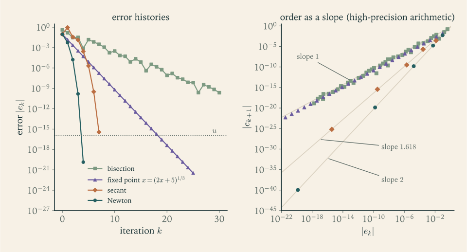
Figure 3.1 puts the methods of the last two chapters on one equation. The fixed-point iteration shown is \(x_{k+1}=(2x_k+5)^{1/3}\) , for which \(g'(r)=2/(3r^2)=0.152\) . In the left panel the two linearly convergent methods are straight lines whose slopes are their rates, and the two superlinear methods bend away from any straight line. The right panel is the diagnostic to use on your own computations: plot \(\log\lvert e_{k+1}\rvert\) against \(\log\lvert e_k\rvert\) and read the order from the slope.
3.6 Failure, and a safeguard
Theorems 3.3 and 3.4 are local, and outside the neighbourhood they describe Newton’s method can do anything.
Divergence. For \(f(x)=\arctan x\) the root is \(0\) and the tangent lines far from the root are nearly horizontal. From \(x_0=1.5\) the iterates are \(-1.694\) , \(2.321\) , \(-5.114\) , \(32.30\) , \(-1575\) : each overshoots further than the last. The boundary case is the starting value from which \(x_1=-x_0\) , which satisfies \(2x=(1+x^2)\arctan x\) and equals \(1.3917\) ; the method converges from \(\lvert x_0\rvert<1.3917\) and diverges from \(\lvert x_0\rvert>1.3917\) .
Cycling. For \(f(x)=x^3-2x+2\) and \(x_0=0\) the tangent at \(0\) crosses zero at \(1\) , and the tangent at \(1\) crosses zero at \(0\) . The iterates are \(0,1,0,1,\dots\) for ever, and starting values near \(0\) are drawn into the same cycle (Exercise 3.11), although the function has a real root near \(-1.77\) .
Vanishing derivative. If \(f'(x_k)=0\) the step is undefined, and if \(f'(x_k)\) is merely small the step is enormous and lands far from anything relevant.
Common mistake. Taking the convergence of Newton’s method for granted because a few steps “looked like they were settling down”, or stopping on a small step without checking the residual. Quadratic convergence has a signature, the doubling of correct digits or equivalently the squaring of successive steps, and its absence means the iteration is not yet, or not at all, in the regime of Theorem 3.4. Linear convergence with ratio near \(\tfrac12\) points to a double root; erratic steps point to a poor starting value. Print the steps and the residuals, compare them with the predicted pattern, and do not report a root until the pattern is there.
The remedy is to keep what Chapter 2 provided. Maintain a bracket \([a,b]\) with a sign change. Compute the Newton step; if it lands strictly inside the bracket, accept it, and otherwise take the midpoint instead. Either way evaluate \(f\) at the new point and shrink the bracket to the side that keeps the sign change.
def safe_newton(f, df, a, b, x, tol):
    fa = f(a)
    while True:
        fx = f(x)
        if fx == 0:
            return x
        if (fx > 0) == (fa > 0):
            a, fa = x, fx
        else:
            b = x
        d = df(x)
        new = x - fx / d if d != 0 else a
        if not (a < new < b):
            new = a + (b - a) / 2
        if abs(new - x) <= tol:
            return new
        x = new
The root can never escape, because it is always inside the bracket, and near a simple root the Newton steps are accepted and the convergence is quadratic.
Example 3.6: Rescuing Newton’s method on the arctangent
Run the listing on \(f(x)=\arctan x\) with bracket \([-2,5]\) and the deliberately bad start \(x_0=5\) . The plain Newton step from \(5\) would go to \(5-26\arctan5=-30.7\) , far outside the bracket, so the midpoint \(1.5\) is taken and the bracket becomes \([-2,1.5]\) . From \(1.5\) the Newton step goes to \(-1.694\) , which is inside the bracket and is accepted, though it is a poor step; the bracket becomes \([-1.694,1.5]\) . From \(-1.694\) Newton proposes \(2.321\) , outside the bracket, and the midpoint \(-0.0970\) is taken. Now the iterate is within the region of fast convergence, and three accepted Newton steps give \(6.08\times10^{-4}\) , \(-1.50\times10^{-10}\) , and \(0\) exactly. The sequence of points is
Two bisection steps were needed, each at a moment when unguarded Newton would have left the interval for good. The cubes of the last errors are visible in the pattern: for the arctangent \(f''(0)=0\) , so the convergence near the root is of third order.
Production root-finders are built on this pattern. The most widely used, Brent’s method, needs no derivative: it keeps a bracket, tries a secant step or a step based on a parabola through three points, and falls back on bisection whenever the fast step is not making the bracket shrink quickly enough. It is guaranteed to converge for any continuous function with a sign change and is superlinear for smooth ones.
3.7 Several equations in several unknowns
For a system \(F(x)=0\)
of \(n\)
equations in \(n\)
unknowns the tangent line becomes the tangent linear map. If \(F\)
is differentiable, then near \(x_k\)
we have \(F(x)\approx F(x_k)+J(x_k)(x-x_k)\)
, where \(J\)
is the Jacobian matrix of partial derivatives \(\partial F_i/\partial x_j\)
, the matrix of the total derivative from Multivariable Calculus (math.multivariable-calculus.total-derivative-chain-rule). Setting the linear model to zero gives Newton’s method for systems:
Each step solves a linear system; the inverse of \(J\)
is never formed. If \(F\)
is twice continuously differentiable and \(J(r)\)
is nonsingular at a root \(r\)
, the iteration converges quadratically from starting points close enough to \(r\)
; the proof follows that of Theorem 3.4 with norms in place of absolute values, and we do not give it. What does not carry over is bracketing. In more than one dimension there is no sign change to trap a root, and making Newton’s method reliable from poor starting points requires other devices, such as shortening the step until \(\lVert F\rVert\)
decreases. When \(F\)
is the gradient of a function to be minimized, those devices and the question of what the limit point is are treated in Continuous Optimization (math.continuous-optimization.newton-quasi-newton).
Example 3.7: A circle meets an exponential curve
Find the intersection of the circle \(x^2+y^2=4\) with the curve \(y=1-e^{x}\) in the fourth quadrant. Put
From the starting point \((1,-1.5)\) :
| \(k\) | \(x_k\) | \(y_k\) | \(\lVert F(x_k,y_k)\rVert_\infty\) |
|---|---|---|---|
| \(0\) | \(1\) | \(-1.5\) | \(7.50\times10^{-1}\) |
| \(1\) | \(1.0093703557\) | \(-1.7437530962\) | \(5.95\times10^{-2}\) |
| \(2\) | \(1.0041994207\) | \(-1.7296844191\) | \(2.25\times10^{-4}\) |
| \(3\) | \(1.0041687391\) | \(-1.7296372876\) | \(3.16\times10^{-9}\) |
| \(4\) | \(1.0041687385\) | \(-1.7296372870\) | below \(10^{-15}\) |
The residual norms satisfy \(2.25\times10^{-4}/(5.95\times10^{-2})^2=0.063\) and \(3.16\times10^{-9}/(2.25\times10^{-4})^2=0.063\) : each is a fixed multiple of the square of the one before, the signature of quadratic convergence. The first step, for instance, solves
whose solution is \(s_0=(0.00937,-0.24375)\) .
The cost of a Newton step for a system is the cost of evaluating \(n^2\) partial derivatives and solving an \(n\times n\) linear system. How to do the latter stably, and what it costs, is the subject of Chapter 7. Before that, the next three chapters turn from equations to functions: how to represent one by finitely many numbers, and what is lost in doing so.
Exercises
-
Show that \(g(x)=e^{-x}\) maps \([0.4,0.7]\) into itself and is a contraction there, give a contraction constant, use the a priori bound to find how many iterations from \(x_0=0.5\) guarantee an error below \(10^{-6}\) , and compare with the asymptotic rate predicted by Theorem 3.3.
Solution
The function \(g(x)=e^{-x}\) is decreasing, so it maps \([0.4,0.7]\) onto \([e^{-0.7},e^{-0.4}]=[0.4966,0.6703]\) , which lies inside \([0.4,0.7]\) . Its derivative satisfies \(\lvert g'(x)\rvert=e^{-x}\le e^{-0.4}=0.6703\) on the interval, so by the mean value theorem \(g\) is a contraction with \(L=0.6703\) , and Theorem 3.2 applies.
From \(x_0=0.5\) the first iterate is \(x_1=e^{-0.5}=0.6065\) , so \(\lvert x_1-x_0\rvert=0.1065\) . The a priori bound requires
\[ \frac{L^{k}}{1-L}\,(0.1065)\le10^{-6}, \]that is, \(k\ge\ln\bigl(10^{-6}(1-L)/0.1065\bigr)/\ln L\) , which gives \(k\ge31.7\) . So \(32\) iterations are guaranteed to suffice.
The fixed point is \(r=0.5671\) , and Theorem 3.3 gives the asymptotic rate \(\lvert g'(r)\rvert=e^{-r}=r=0.5671\) , noticeably smaller than \(L\) . The actual iteration is correspondingly faster than the guarantee: an error below \(10^{-6}\) is reached at \(k=20\) . The a priori bound is safe but uses the worst contraction factor on the interval.
-
The equation \(x^3+x-1=0\) has the root \(r=0.6823\) . For each rearrangement decide by Theorem 3.3 whether the fixed-point iteration converges locally and give the rate when it does: (a) \(g(x)=1-x^3\) ; (b) \(g(x)=(1-x)^{1/3}\) ; (c) \(g(x)=1/(1+x^2)\) .
Answer
(a) \(g'(r)=-3r^2=-1.397\) : the fixed point repels, no convergence. (b) \(g'(r)=-\tfrac13(1-r)^{-2/3}=-1/(3r^2)=-0.716\) , using \(1-r=r^3\) : local linear convergence with rate \(0.716\) . (c) \(g'(r)=-2r/(1+r^2)^2=-2r^3=-0.635\) , using \(1/(1+r^2)=r\) : local linear convergence with rate \(0.635\) . Both convergent iterations alternate about the root because \(g'(r)<0\) .
-
Prove part (c) of Theorem 3.3: if \(g\) is continuously differentiable near a fixed point \(r\) and \(\lvert g'(r)\rvert>1\) , then a fixed-point iteration can converge to \(r\) only if some iterate equals \(r\) exactly.
Solution
Put \(L'=\tfrac12(1+\lvert g'(r)\rvert)\) , so that \(1<L'<\lvert g'(r)\rvert\) . Since \(g'\) is continuous at \(r\) , there is a \(\delta>0\) such that \(\lvert g'(x)\rvert\ge L'\) whenever \(\lvert x-r\rvert\le\delta\) .
Suppose, for contradiction, that \(x_k\to r\) while \(e_k=x_k-r\ne0\) for every \(k\) . Convergence means there is an index \(K\) with \(\lvert e_k\rvert\le\delta\) for all \(k\ge K\) . For such \(k\) the mean value theorem gives a point \(\xi_k\) between \(x_k\) and \(r\) , hence within \(\delta\) of \(r\) , with
\[ e_{k+1}=g(x_k)-g(r)=g'(\xi_k)\,e_k,\qquad\text{so}\qquad\lvert e_{k+1}\rvert\ge L'\lvert e_k\rvert . \]By induction \(\lvert e_k\rvert\ge(L')^{k-K}\lvert e_K\rvert\) for all \(k\ge K\) . Since \(L'>1\) and \(e_K\ne0\) , the right side tends to infinity, contradicting \(\lvert e_k\rvert\le\delta\) . Therefore convergence to \(r\) is possible only if \(e_k=0\) for some \(k\) , that is, some iterate lands exactly on \(r\) , after which all later iterates equal \(r\) .
-
Carry out two steps of Newton’s method for \(f(x)=x^2-5\) from \(x_0=2\) in exact fractions, compute the errors of \(x_1\) and \(x_2\) , and check that \(e_{k+1}/e_k^2\) is close to the constant predicted by Theorem 3.4.
Solution
Newton’s iteration for \(x^2-5\) is \(x_{k+1}=\tfrac12(x_k+5/x_k)\) . From \(x_0=2\) ,
\[ x_1=\tfrac12\Bigl(2+\tfrac52\Bigr)=\frac94=2.25,\qquad x_2=\tfrac12\Bigl(\frac94+\frac{20}{9}\Bigr)=\frac{161}{72}=2.236111 . \]With \(\sqrt5=2.2360680\) , the errors are \(e_0=-0.23607\) , \(e_1=1.3932\times10^{-2}\) , and \(e_2=4.313\times10^{-5}\) . The ratios \(e_{k+1}/e_k^2\) are \(0.2500\) and \(0.2222\) . Theorem 3.4 predicts the limit \(f''(r)/(2f'(r))=2/(4\sqrt5)=1/(2\sqrt5)=0.2236\) , and the ratios bracket it.
For this function the relation is exact at every step: from the proof of Theorem 3.4 with \(f''\equiv2\) , \(e_{k+1}=e_k^2/(2x_k)\) , so the ratios are \(1/(2x_0)=\tfrac14\) and \(1/(2x_1)=\tfrac29\) , tending to \(1/(2\sqrt5)\) as \(x_k\to\sqrt5\) . As a check on the fraction, \(x_2^2-5=1/5184\) , a residual of \(1.9\times10^{-4}\) , which divided by the slope \(2\sqrt5\) gives the error \(4.3\times10^{-5}\) in agreement with Proposition 2.4.
-
Apply Newton’s method to \(f(x)=1/x-a\) with \(a>0\) and show that the iteration is \(x_{k+1}=x_k(2-ax_k)\) , which uses no division; prove that \(e_{k+1}=-a\,e_k^2\) exactly and that the iteration converges to \(1/a\) if and only if \(0<x_0<2/a\) .
Solution
With \(f(x)=1/x-a\) we have \(f'(x)=-1/x^2\) , so
\[ x-\frac{f(x)}{f'(x)}=x+x^2\Bigl(\frac1x-a\Bigr)=2x-ax^2=x(2-ax), \]which involves only multiplication and subtraction.
Error recursion. With \(e_k=x_k-1/a\) ,
\[ -a\,e_k^2=-a\Bigl(x_k^2-\frac{2x_k}{a}+\frac1{a^2}\Bigr)=2x_k-ax_k^2-\frac1a=x_{k+1}-\frac1a=e_{k+1}. \]Convergence. Multiply by \(a\) : the scaled error \(\rho_k=a\,e_k=ax_k-1\) satisfies \(\rho_{k+1}=-\rho_k^2\) , so \(\lvert\rho_k\rvert=\lvert\rho_0\rvert^{2^{k}}\) . This tends to zero if and only if \(\lvert\rho_0\rvert<1\) , that is, \(\lvert ax_0-1\rvert<1\) , that is, \(0<x_0<2/a\) . If \(\lvert\rho_0\rvert=1\) then \(x_0=0\) or \(x_0=2/a\) , and in both cases \(x_1=0\) and the iteration stays at \(0\) . If \(\lvert\rho_0\rvert>1\) the scaled errors grow without bound. Hence the iteration converges to \(1/a\) exactly when \(0<x_0<2/a\) , and then quadratically. This iteration is how division was implemented on machines that had only a multiplier.
-
Derive the Newton iteration for the cube root of \(a\) from \(f(x)=x^3-a\) , carry out three steps for \(a=10\) from \(x_0=2\) , and give the asymptotic error constant.
Answer
\(x_{k+1}=x_k-(x_k^3-a)/(3x_k^2)=\tfrac13(2x_k+a/x_k^2)\) . For \(a=10\) and \(x_0=2\) : \(x_1=2.1666667\) , \(x_2=2.1545036\) , \(x_3=2.1544347\) , against \(10^{1/3}=2.15443469\) . The asymptotic constant is \(f''(r)/(2f'(r))=6r/(6r^2)=1/r=0.464\) .
-
Newton’s method applied to \(f(x)=e^{x}-x-1\) from \(x_0=1\) produces iterates \(0.5820\) , \(0.3191\) , \(0.1680\) , \(0.0863\) . Explain why the errors only halve at each step, identify the multiplicity of the root, and give a modification that restores quadratic convergence together with its first two iterates.
Solution
The root is \(x=0\) . There \(f(0)=e^{0}-0-1=0\) and \(f'(0)=e^{0}-1=0\) , while \(f''(0)=1\ne0\) . So \(0\) is a double root: \(f(x)=x^2h(x)\) with \(h(0)=\tfrac12\) . Theorem 3.4 does not apply, because it requires \(f'(r)\ne0\) , and Proposition 3.6 with \(m=2\) says that Newton’s method converges linearly with rate \(1-\tfrac12=\tfrac12\) . Since the root is \(0\) the iterates are their own errors, and the given values have ratios \(0.5820\) , \(0.5482\) , \(0.5265\) , \(0.5140\) , approaching \(\tfrac12\) ; three more steps give a ratio of \(0.502\) .
The modification is to multiply the Newton correction by the multiplicity: \(x_{k+1}=x_k-2f(x_k)/f'(x_k)\) . From \(x_0=1\) this gives
\[ x_1=1-\frac{2(e-2)}{e-1}=0.1640,\qquad x_2=0.00448, \]so the first two modified iterates are \(0.1640\) and \(0.00448\) , and the next is \(3.3\times10^{-6}\) : the exponent now doubles. A caution carries over from Example 3.4: the numerator \(e^{x}-x-1\) suffers cancellation for small \(x\) , so the attainable accuracy for this double root, with \(f\) evaluated as written, is only about \(\sqrt u\approx10^{-8}\) .
-
Carry out two steps of the secant method for \(f(x)=x^2-5\) from \(x_0=2\) and \(x_1=3\) , giving \(x_2\) and \(x_3\) as fractions, and compare the error of \(x_3\) with that of the Newton iterate \(x_2\) of Exercise 3.4 in terms of function evaluations used.
Answer
\(x_2=3-4\cdot(3-2)/(4-(-1))=\tfrac{11}{5}=2.2\) , where \(f=-0.16\) ; then \(x_3=2.2-(-0.16)(2.2-3)/(-0.16-4)=\tfrac{29}{13}=2.230769\) , with error \(-5.3\times10^{-3}\) . This used three function evaluations. Newton’s \(x_2\) , with error \(4.3\times10^{-5}\) , used four (two of \(f\) , two of \(f'\) ). One more secant step, a fourth evaluation, gives \(x_4=2.236111\) with error \(4.3\times10^{-5}\) : the same accuracy for the same number of evaluations on this problem.
-
Suppose the errors of an iteration satisfy \(\lvert e_{k+1}\rvert=C\lvert e_k\rvert\lvert e_{k-1}\rvert\) and also \(\lvert e_{k+1}\rvert=A\lvert e_k\rvert^{p}\) for all large \(k\) . Show that \(p^2=p+1\) and that \(A=C^{1/p}\) .
Solution
From \(\lvert e_k\rvert=A\lvert e_{k-1}\rvert^{p}\) solve for the older error: \(\lvert e_{k-1}\rvert=(\lvert e_k\rvert/A)^{1/p}\) . Substitute into the product relation:
\[ \lvert e_{k+1}\rvert=C\,\lvert e_k\rvert\,\lvert e_{k-1}\rvert=C\,A^{-1/p}\,\lvert e_k\rvert^{\,1+1/p}. \]This must agree with \(\lvert e_{k+1}\rvert=A\lvert e_k\rvert^{p}\) for all large \(k\) , along a sequence of errors tending to zero. Two power laws in \(\lvert e_k\rvert\) agree for arbitrarily small arguments only if their exponents and their coefficients agree. Equating exponents, \(p=1+1/p\) , that is, \(p^2=p+1\) , whose positive root is \(p=\tfrac12(1+\sqrt5)\) . Equating coefficients, \(A=C\,A^{-1/p}\) , so \(A^{1+1/p}=C\) . Since \(1+1/p=p\) , this reads \(A^{p}=C\) , that is, \(A=C^{1/p}\) . For the cubic of Example 3.5, \(C=0.5630\) and \(A=0.5630^{0.618}=0.701\) .
-
The efficiency index of a method of order \(p\) that uses \(m\) function evaluations per step is \(p^{1/m}\) . Compute it for Newton’s method, for the secant method, and for a third-order method that uses three evaluations per step, and say how the comparison between Newton and secant changes when \(f'\) costs only one fifth as much as \(f\) .
Answer
Newton: \(2^{1/2}=1.414\) . Secant: \(1.618^{1/1}=1.618\) . Third-order method with three evaluations: \(3^{1/3}=1.442\) . The secant method is the most efficient of the three when all evaluations cost the same. If \(f'\) costs one fifth of \(f\) , a Newton step costs \(1.2\) evaluations of \(f\) and its index is \(2^{1/1.2}=1.78\) , which beats the secant method.
-
Verify that Newton’s method for \(f(x)=x^3-2x+2\) from \(x_0=0\) produces the cycle \(0,1,0,1,\dots\) , and show, by computing the derivative of the Newton map \(g\) at \(0\) and at \(1\) , that starting values close to \(0\) are attracted to this cycle.
Solution
The Newton map is \(g(x)=x-(x^3-2x+2)/(3x^2-2)\) . At \(x=0\) : \(f(0)=2\) and \(f'(0)=-2\) , so \(g(0)=0-2/(-2)=1\) . At \(x=1\) : \(f(1)=1\) and \(f'(1)=1\) , so \(g(1)=1-1=0\) . Hence the iterates from \(x_0=0\) are \(0,1,0,1,\dots\)
For the stability of the cycle, look at the map applied twice, \(G=g\circ g\) . Both \(0\) and \(1\) are fixed points of \(G\) . By the chain rule \(G'(0)=g'(g(0))\,g'(0)=g'(1)\,g'(0)\) . For any Newton map \(g'(x)=f(x)f''(x)/f'(x)^2\) . Here \(f''(x)=6x\) , so \(g'(0)=f(0)\cdot0/4=0\) and \(g'(1)=1\cdot6/1=6\) . Therefore \(G'(0)=6\cdot0=0\) , and likewise \(G'(1)=g'(0)g'(1)=0\) .
Since \(\lvert G'(0)\rvert<1\) , Theorem 3.3(a) applied to \(G\) says that the iteration \(x_{k+2}=G(x_k)\) converges to \(0\) from every starting value close enough to \(0\) ; in fact quadratically, by part (b), since \(G'(0)=0\) . So for \(x_0\) near \(0\) the even-numbered Newton iterates converge to \(0\) and the odd-numbered ones to \(g(0)=1\) : the starting value is drawn into the cycle and never approaches the real root near \(-1.77\) .
-
For \(f(x)=\arctan x\) , derive the equation satisfied by the starting value \(x_0>0\) for which Newton’s method gives \(x_1=-x_0\) , explain why this value separates convergence from divergence, and locate it to two decimal places by bisection.
Hint
Write \(x_1=x_0-(1+x_0^2)\arctan x_0\) and set \(x_1=-x_0\) . Because \(\arctan\) is odd, a start with \(x_1=-x_0\) gives \(x_2=x_0\) , a cycle of period two. Starts inside the cycle are pulled inward, those outside pushed outward; argue this from the sign of \(2x-(1+x^2)\arctan x\) on either side of its zero. That function is positive at \(1\) and negative at \(2\) , and bisection gives \(1.39\) .
-
Prove that Newton’s iteration \(x_{k+1}=\tfrac12(x_k+a/x_k)\) for \(\sqrt a\) with \(a>0\) converges from every \(x_0>0\) , by showing that \(x_1\ge\sqrt a\) and then applying Proposition 3.5.
Solution
Let \(r=\sqrt a\) and \(x_0>0\) . The first iterate satisfies
\[ x_1-\sqrt a=\tfrac12\Bigl(x_0+\frac{a}{x_0}\Bigr)-\sqrt a=\frac{x_0^2-2\sqrt a\,x_0+a}{2x_0}=\frac{(x_0-\sqrt a)^2}{2x_0}\ge0, \]so \(x_1\ge\sqrt a\) whatever positive \(x_0\) was chosen.
Now apply Proposition 3.5 on the interval \(I=(0,\infty)\) to \(f(x)=x^2-a\) . There \(f'(x)=2x>0\) and \(f''(x)=2\ge0\) , the root \(\sqrt a\) lies in \(I\) , and the starting value \(x_1\) lies in \(I\) with \(x_1\ge r\) . The proposition gives \(\sqrt a\le x_{k+1}\le x_k\) for all \(k\ge1\) and \(x_k\to\sqrt a\) . So the iteration converges from every positive start: after at most one step the iterates are on the right of the root and decrease monotonically to it. Once they are close, Theorem 3.4 takes over and the convergence is quadratic, with \(e_{k+1}=e_k^2/(2x_k)\) exactly, as the displayed identity shows.
-
On a convex function with \(f(a)<0<f(b)\) , false position keeps \(b\) fixed and updates the left endpoint by \(g(x)=x-f(x)(b-x)/(f(b)-f(x))\) . Compute \(g'(r)\) , deduce from Theorem 3.3 the rate of convergence stated in Section 2.5, and evaluate it for \(f(x)=x^{10}-1\) on \([0,1.3]\) .
Solution
Differentiate \(g(x)=x-f(x)(b-x)/(f(b)-f(x))\) by the product and quotient rules:
\[ g'(x)=1-\frac{\bigl(f'(x)(b-x)-f(x)\bigr)\bigl(f(b)-f(x)\bigr)+f(x)(b-x)f'(x)}{\bigl(f(b)-f(x)\bigr)^2}. \]At \(x=r\) every term containing the factor \(f(r)=0\) drops out, leaving
\[ g'(r)=1-\frac{f'(r)\,(b-r)}{f(b)} . \]Also \(g(r)=r\) , so \(r\) is a fixed point of the update map. For a convex function the graph lies above its tangent at \(r\) , so \(f(b)\ge f'(r)(b-r)\) , and \(f'(r)>0\) because \(f\) passes from negative to positive values at \(r\) . Hence \(0\le g'(r)<1\) , and Theorem 3.3(a) gives local convergence of the moving endpoint, linear with rate \(g'(r)\) whenever \(g'(r)\ne0\) , which is the case unless the graph coincides with its tangent between \(r\) and \(b\) . This is the rate \(C\) stated in Section 2.5.
For \(f(x)=x^{10}-1\) , \(r=1\) , and \(b=1.3\) : \(f'(1)=10\) , \(b-r=0.3\) , and \(f(b)=12.786\) , so \(g'(r)=1-3/12.786=0.7654\) , matching the observed ratio in Example 2.5.
-
An iteration is stopped when \(\lvert x_{k+1}-x_k\rvert\le10^{-6}\) . Estimate the error of \(x_{k+1}\) when the convergence is linear with rate \(0.9\) and when it is quadratic, and say which stopping rule from Theorem 3.2 should be used in the linear case.
Answer
Linear, rate \(0.9\) : \(x_{k+1}-x_k\approx(C-1)e_k\) , so \(\lvert e_{k+1}\rvert\approx C\lvert e_k\rvert\approx\tfrac{C}{1-C}\lvert x_{k+1}-x_k\rvert=9\times10^{-6}\) , nine times the step. Quadratic: the step is about \(\lvert e_k\rvert=10^{-6}\) and \(\lvert e_{k+1}\rvert\approx M\lvert e_k\rvert^2\) , of order \(10^{-12}\) . In the linear case use the a posteriori bound \(\tfrac{L}{1-L}\lvert x_k-x_{k-1}\rvert\) of Theorem 3.2, with \(L\) estimated from the ratio of successive steps.
-
The chord method freezes the derivative: \(x_{k+1}=x_k-f(x_k)/d\) with \(d=f'(x_0)\) . Show that it converges locally with linear rate \(\lvert1-f'(r)/d\rvert\) , and compute the rate for \(f(x)=x^3-2x-5\) with \(x_0=2\) , comparing with the errors of the first few iterates.
Solution
The chord method is the fixed-point iteration for \(g(x)=x-f(x)/d\) with \(d\) a fixed nonzero number. A root \(r\) of \(f\) is a fixed point of \(g\) , and \(g'(r)=1-f'(r)/d\) . By Theorem 3.3(a) the iteration converges locally when \(\lvert1-f'(r)/d\rvert<1\) , linearly with that rate unless \(d=f'(r)\) exactly. With \(d=f'(x_0)\) and \(x_0\) near \(r\) the rate is small, because \(f'(x_0)\approx f'(r)\) , but it is not zero: freezing the derivative trades quadratic convergence for linear convergence with a small rate, and saves all derivative evaluations after the first.
For \(f(x)=x^3-2x-5\) and \(x_0=2\) : \(d=f'(2)=10\) and \(f'(r)=3r^2-2=11.161\) , so the predicted rate is \(\lvert1-11.161/10\rvert=0.1161\) . The chord iterates have errors \(9.455\times10^{-2}\) , \(5.449\times10^{-3}\) , \(6.515\times10^{-4}\) , \(7.540\times10^{-5}\) , \(8.761\times10^{-6}\) , with ratios \(0.0576\) , \(0.1196\) , \(0.1157\) , \(0.1162\) . The first step coincides with Newton’s and is unusually good; after that each step gains a little less than one decimal digit, as the rate \(0.116\) predicts.
-
In Example 3.4 Newton’s method stalls with an error near \(10^{-8}\) . Using Proposition 1.5 and Section 2.3, explain why no method that uses only double-precision values of \(x^3-3x+2\) can do substantially better, and say how \(f\) could be evaluated to locate the root to full precision.
Hint
The terms \(x^3\) , \(3x\) , and \(2\) have magnitudes \(1\) , \(3\) , \(2\) near the root; bound the evaluation error by Proposition 1.5 and compare it with \(f(x)\approx3(x-1)^2\) . For the remedy, think of Example 2.3: which form of \(f\) has a small relative error for every \(x\) near \(1\) ?
-
For the system \(x^2+y^2=1\) , \(y=x^2\) , write \(F\) and its Jacobian, carry out one Newton step by hand from \((1,1)\) , and give the second iterate; compare with the exact solution \(y=\tfrac12(\sqrt5-1)\) , \(x=\sqrt y\) .
Solution
Write the system as \(F(x,y)=0\) with
\[ F(x,y)=\begin{pmatrix}x^2+y^2-1\\ y-x^2\end{pmatrix},\qquad J(x,y)=\begin{pmatrix}2x&2y\\-2x&1\end{pmatrix}. \]At \((1,1)\) : \(F=(1,0)\) and \(J=\begin{pmatrix}2&2\\-2&1\end{pmatrix}\) . The Newton step solves \(2s_1+2s_2=-1\) and \(-2s_1+s_2=0\) . The second equation gives \(s_2=2s_1\) , and then \(6s_1=-1\) , so \(s=(-\tfrac16,-\tfrac13)\) and
\[ (x_1,y_1)=(5/6,\,2/3). \]At this point \(F=(\tfrac{25}{36}+\tfrac49-1,\ \tfrac23-\tfrac{25}{36})=(\tfrac5{36},-\tfrac1{36})\) , and solving the next linear system in exact fractions gives
\[ (x_2,y_2)=(331/420,\,13/21)=(0.78810,\,0.61905). \]The exact solution is \(y=\tfrac12(\sqrt5-1)=0.61803\) and \(x=\sqrt y=0.78615\) . The errors in \(x\) are \(0.214\) , \(0.047\) , and \(0.0019\) for the three points: roughly squared at each step once the iterates are close, as quadratic convergence requires. Two more steps reduce the residual to \(7\times10^{-12}\) .
-
A program applies Newton’s method to \(f(x)=10^{-8}(x^2-2)\) and stops as soon as \(\lvert f(x_k)\rvert<10^{-9}\) . Say what it returns from \(x_0=1.5\) , explain why the test is at fault, and propose a stopping test that does not depend on how \(f\) is scaled.
Answer
\(\lvert f(1.5)\rvert=2.5\times10^{-9}\) exceeds the threshold, so one Newton step is taken, to \(x_1=1.41667\) , where \(\lvert f\rvert=6.9\times10^{-11}<10^{-9}\) . The program returns \(1.41667\) , wrong in the third decimal. Multiplying \(f\) by a constant does not change its roots or the Newton iterates, but it changes the residual, so an absolute residual test is meaningless without a scale. Test the step relative to the iterate, \(\lvert x_{k+1}-x_k\rvert\le\tau\lvert x_{k+1}\rvert\) , or the residual relative to a natural scale such as \(\lvert f(x_0)\rvert\) or the sum of the magnitudes of the terms of \(f\) .
-
The safeguarded iteration of Section 3.6 accepts any Newton step that lands inside the bracket. Describe a function and bracket for which accepted steps shrink the bracket only slowly, as in Section 2.5, and explain how requiring each accepted step to at least halve the bracket length over two iterations would bound the total number of steps.
Hint
Consider \(f(x)=x^{10}-1\) on \([0,1.3]\) started at \(x=1.3\) : every Newton iterate stays to the right of the root (Proposition 3.5), is accepted, and replaces the right endpoint, while the left endpoint \(0\) never moves, so the bracket length stays above \(1\) . The iteration still converges here, but nothing in the acceptance rule bounds the work. If a bisection is forced whenever two accepted steps fail to halve the bracket, the length at least halves every three evaluations, and the count is at most three times that of bisection.