A system of \(N\) linear equations in \(N\) unknowns, \(Kc=F\) , has exactly one solution for every right side if the matrix is positive definite, meaning \(c^{\top}Kc>0\) for every nonzero \(c\) . The proof takes two lines: positive definiteness makes \(Kc=0\) impossible for \(c\ne0\) , so \(K\) is injective, and an injective linear map of a finite-dimensional space into itself is surjective. Every weak formulation of Chapter 9 looked like such a system, with the space \(H_0^1\) or \(H^1\) in place of \(\mathbb R^N\) , and the uniqueness proofs there were the first of those two lines: test with the solution itself and use positivity. The second line is where infinite dimensions bite. An injective linear map of an infinite-dimensional space into itself need not be surjective. What replaces counting dimensions?
The answer is completeness together with a quantitative form of positivity. With those two properties the existence of weak solutions becomes a theorem of functional analysis, which this chapter applies. The same structure yields a practical method of computing approximations, by restricting the problem to a finite-dimensional subspace, where it is again a positive definite linear system. The chapter ends by setting the methods of the whole book side by side.
10.1 The abstract problem and the Lax–Milgram theorem
Definition 10.1 (bounded and coercive forms). Let \(V\) be a real Hilbert space with norm \(\lVert\cdot\rVert_V\) . A bilinear form \(a:V\times V\to\mathbb R\) is bounded if there is a constant \(M\) with \(\lvert a(u,v)\rvert\le M\lVert u\rVert_V\lVert v\rVert_V\) for all \(u,v\) , and coercive if there is a constant \(\alpha>0\) with
A linear functional \(\ell:V\to\mathbb R\) is bounded if \(\lvert\ell(v)\rvert\le\Lambda\lVert v\rVert_V\) for some \(\Lambda\) and all \(v\) ; the smallest such \(\Lambda\) is written \(\lVert\ell\rVert_{V'}\) .
The abstract variational problem is: find \(u\in V\) such that \(a(u,v)=\ell(v)\) for all \(v\in V\) .
Theorem 10.2 (Lax–Milgram). Let \(V\) be a real Hilbert space, \(a\) a bounded, coercive bilinear form on \(V\) , and \(\ell\) a bounded linear functional on \(V\) . Then the abstract variational problem has exactly one solution \(u\) , and
The theorem belongs to Functional Analysis, where it is proved (math.functional-analysis.lax-milgram-theorem); we use it without reproducing the proof. It is worth separating what is easy in it from what is not. Uniqueness and the estimate are easy and are the argument of Theorem 9.9: if \(u\)
is a solution, then \(\alpha\lVert u\rVert_V^2\le a(u,u)=\ell(u)\le\lVert\ell\rVert_{V'}\lVert u\rVert_V\)
, and the difference of two solutions solves the problem with \(\ell=0\)
. Existence is the content. When \(a\)
is symmetric it has a short explanation: \(a(\cdot,\cdot)\)
is then itself an inner product on \(V\)
, and boundedness and coercivity say that its norm is equivalent to \(\lVert\cdot\rVert_V\)
, so \(V\)
is complete with respect to it; the claim is then exactly the Riesz representation theorem, that every bounded linear functional on a Hilbert space is the inner product with some element. In that case the solution also minimizes \(\tfrac12a(v,v)-\ell(v)\)
, as in Theorem 9.10. For a form that is not symmetric there is no energy to minimize and the full theorem is needed.
Note the role of each hypothesis. Completeness of \(V\) is what Chapter 9 was built to provide. Boundedness makes the problem meaningful and stable. Coercivity is positive definiteness with a uniform constant: it is not enough that \(a(v,v)>0\) for \(v\ne0\) , because in infinite dimensions \(a(v,v)/\lVert v\rVert_V^2\) could approach zero along a sequence, and the estimate \(\lVert u\rVert\le\lVert\ell\rVert/\alpha\) would then fail.
10.2 Existence of weak solutions
Theorem 10.3 (the Dirichlet problem is well-posed in the energy space). Let \(\Omega\subset\mathbb R^n\) be a bounded open set and \(f\in L^2(\Omega)\) . There is exactly one weak solution \(u\in H_0^1(\Omega)\) of \(-\Delta u=f\) in \(\Omega\) , \(u=0\) on \(\partial\Omega\) . It satisfies \(\lVert\nabla u\rVert\le C_P\lVert f\rVert\) , and the map \(f\mapsto u\) is linear.
Proof. We verify the hypotheses of Theorem 10.2 with \(V=H_0^1(\Omega)\) , \(\lVert\cdot\rVert_V=\lVert\cdot\rVert_{H^1}\) , \(a(u,v)=\int_\Omega\nabla u\cdot\nabla v\,dx\) , and \(\ell(v)=\int_\Omega fv\,dx\) .
Hilbert space. \(H^1(\Omega)\) is complete by Theorem 9.2 and \(H_0^1(\Omega)\) is a closed subspace by its definition.
Boundedness of the form. By the Cauchy–Schwarz inequality, \(\lvert a(u,v)\rvert\le\lVert\nabla u\rVert\,\lVert\nabla v\rVert\le\lVert u\rVert_{H^1}\lVert v\rVert_{H^1}\) ; so \(M=1\) .
Coercivity of the form. Since \(\Omega\) is bounded it lies in a slab, and the Poincaré inequality, Theorem 9.6, gives \(\lVert v\rVert_{H^1}^2\le(1+C_P^2)\lVert\nabla v\rVert^2\) for \(v\in H_0^1(\Omega)\) . Hence \(a(v,v)=\lVert\nabla v\rVert^2\ge\alpha\lVert v\rVert_{H^1}^2\) with \(\alpha=1/(1+C_P^2)\) .
Boundedness of the functional. \(\lvert\ell(v)\rvert\le\lVert f\rVert\,\lVert v\rVert\le\lVert f\rVert\,\lVert v\rVert_{H^1}\) .
Theorem 10.2 now gives a unique \(u\in H_0^1(\Omega)\) with \(a(u,v)=\ell(v)\) for all \(v\in H_0^1(\Omega)\) , which is Definition 9.7. The estimate is Theorem 9.9, and linearity of \(f\mapsto u\) follows from uniqueness.
Consider what has been proved and at what cost. For every bounded open set, with no assumption whatever on its boundary, and every square-integrable load, the Dirichlet problem has a solution, it is unique, and it depends continuously on the load: the problem is well-posed in the sense of Definition 1.4. Chapter 4 obtained existence only for a ball and a half-space, by explicit formulas. The cost is that the solution is known only to lie in \(H_0^1\) . Whether it is a classical solution is the question of regularity, which is separate and harder, and which we only report. If \(f\) is infinitely differentiable in \(\Omega\) , then so is \(u\) there. If moreover the boundary is smooth and \(f\) is smooth on the closed region \(\overline\Omega\) , then \(u\) is smooth up to the boundary and is the classical solution; smoothness of \(f\) inside \(\Omega\) alone is not enough for that, as the load \(f=x^{-1/4}\) on \((0,1)\) shows, for which \(u''=-f\) is unbounded at the left end; if the boundary is \(C^2\) or \(\Omega\) is convex, and \(f\in L^2\) , then \(u\) has square-integrable weak second derivatives. At a re-entrant corner of a polygon, on the other hand, the weak solution exists and is unique, but its gradient is in general unbounded near the corner. The weak theory separates two questions that the classical theory had to answer at once: whether a solution exists, and how smooth it is.
The verification extends to operators with variable coefficients and lower-order terms.
Theorem 10.4 (elliptic problems in divergence form). Let \(\Omega\) be a bounded open set. Let \(A(x)\) be an \(n\times n\) matrix of bounded measurable functions with \(\xi^{\top}A(x)\xi\ge\theta\lvert\xi\rvert^2\) and \(\lvert A(x)\xi\rvert\le\Theta\lvert\xi\rvert\) for all \(x\in\Omega\) and \(\xi\in\mathbb R^n\) , where \(\theta>0\) ; let \(\mathbf b\) be a bounded measurable vector field with \(\lvert\mathbf b\rvert\le\beta\) ; let \(c\) be a bounded measurable function with \(0\le c\le\gamma\) ; and let \(f\in L^2(\Omega)\) . If \(\beta C_P<\theta\) , there is exactly one \(u\in H_0^1(\Omega)\) with
and \(\lVert\nabla u\rVert\le\dfrac{C_P}{\theta-\beta C_P}\lVert f\rVert\) .
Proof. The space and the functional are as in Theorem 10.3. For boundedness, \(\lvert a(u,v)\rvert\le\Theta\lVert\nabla u\rVert\lVert\nabla v\rVert+\beta\lVert\nabla u\rVert\lVert v\rVert+\gamma\lVert u\rVert\lVert v\rVert\le(\Theta+\beta+\gamma)\lVert u\rVert_{H^1}\lVert v\rVert_{H^1}\) . For coercivity, using \(c\ge0\) and the Poincaré inequality,
Theorem 10.2 applies. For the estimate, \((\theta-\beta C_P)\lVert\nabla u\rVert^2\le a(u,u)=(f,u)\le C_P\lVert f\rVert\,\lVert\nabla u\rVert\) .
This is the weak form of \(-\nabla\cdot(A\nabla u)+\mathbf b\cdot\nabla u+cu=f\) with zero boundary values: diffusion with conductivity matrix \(A\) , transport by the field \(\mathbf b\) , and absorption at the rate \(c\) . The condition \(\xi^{\top}A\xi\ge\theta\lvert\xi\rvert^2\) is uniform ellipticity; it is the quantitative version of the definition of elliptic type in Section 1.4. When \(\mathbf b\ne0\) the form is not symmetric. The hypothesis \(\beta C_P<\theta\) says that transport is weak compared with diffusion; it is sufficient, not necessary (Exercise 5).
Example 10.1: Coercivity lost at an eigenvalue
On \(V=H_0^1(0,1)\) consider \(-u''-\lambda u=f\) , that is, \(a_\lambda(u,v)=\int_0^1u'v'\,dx-\lambda\int_0^1uv\,dx\) , for a real parameter \(\lambda\) . For \(\lambda\le0\) clearly \(a_\lambda(v,v)\ge\lVert v'\rVert^2\) . For \(0\le\lambda<\pi^2\) the sharp Poincaré inequality \(\lVert v\rVert^2\le\pi^{-2}\lVert v'\rVert^2\) gives
So the form is coercive for every \(\lambda<\pi^2\) , and for \(0\le\lambda<\pi^2\) the weak solution satisfies \(\lVert u'\rVert\le\dfrac{\pi}{\pi^2-\lambda}\lVert f\rVert\) .
Take \(f=\sin(\pi x)\) . The solution is \(u=\dfrac{\sin(\pi x)}{\pi^2-\lambda}\) , since \(-u''=\pi^2u\) . For \(\lambda=5\) its midpoint value is \(1/(\pi^2-5)\approx0.2054\) ; for \(\lambda=9\) it is \(1/(\pi^2-9)\approx1.150\) . As \(\lambda\) increases to \(\pi^2\approx9.870\) the solution grows without bound, exactly as the stability constant \(1/\alpha\) predicts; for this load the estimate above holds with equality.
At \(\lambda=\pi^2\) coercivity fails: \(a_{\pi^2}(\sin\pi x,\sin\pi x)=\tfrac{\pi^2}{2}-\pi^2\cdot\tfrac12=0\) . Both conclusions of the theorem fail with it. The function \(\sin(\pi x)\) solves the problem with \(f=0\) , so solutions are not unique. And for \(f=\sin(\pi x)\) there is no solution: testing with \(v=\sin(\pi x)\) and integrating by parts gives \(a_{\pi^2}(u,\sin\pi x)=0\) for every \(u\in H_0^1(0,1)\) , while the right side is \(\int_0^1\sin^2(\pi x)\,dx=\tfrac12\) . The number \(\pi^2\) is the first eigenvalue of Lemma 7.1; coercivity of \(a_\lambda\) is the statement that \(\lambda\) lies below the spectrum.
10.3 Galerkin’s method
The abstract problem asks for an identity to hold for all \(v\) in an infinite-dimensional space. Galerkin’s idea is to ask for it only on a finite-dimensional subspace, and to look for the solution in that same subspace.
Let \(V_h\subset V\) be a subspace with basis \(\phi_1,\dots,\phi_N\) . The Galerkin approximation is the function \(u_h\in V_h\) with
Writing \(u_h=\sum_jc_j\phi_j\) and testing with \(v=\phi_i\) for each \(i\) turns this into the linear system
For historical reasons \(K\) is called the stiffness matrix and \(F\) the load vector.
Theorem 10.5 (Galerkin approximation). Under the hypotheses of Theorem 10.2, let \(u\) be the solution of the abstract problem and \(V_h\) a finite-dimensional subspace of \(V\) .
(a) The matrix \(K\) is invertible, so the Galerkin approximation \(u_h\) exists and is unique.
(b) Galerkin orthogonality: \(a(u-u_h,v)=0\) for all \(v\in V_h\) .
(c) Céa’s lemma: \(\lVert u-u_h\rVert_V\le\dfrac{M}{\alpha}\,\lVert u-v\rVert_V\) for every \(v\in V_h\) .
(d) If \(a\) is symmetric, with energy norm \(\lVert v\rVert_a=a(v,v)^{1/2}\) , then \(u_h\) is the best approximation to \(u\) from \(V_h\) in the energy norm, and \(\lVert u-u_h\rVert_a^2=\lVert u\rVert_a^2-\lVert u_h\rVert_a^2\) .
Proof. (a) For a coefficient vector \(c\ne0\) put \(v=\sum c_j\phi_j\) , which is not zero because the \(\phi_j\) are linearly independent. Then \(c^{\top}Kc=a(v,v)\ge\alpha\lVert v\rVert_V^2>0\) . So \(Kc=0\) only for \(c=0\) , and a square matrix with trivial null space is invertible.
(b) Subtract \(a(u_h,v)=\ell(v)\) from \(a(u,v)=\ell(v)\) , both valid for \(v\in V_h\) .
(c) Let \(v\in V_h\) . Since \(v-u_h\in V_h\) , part (b) gives \(a(u-u_h,v-u_h)=0\) , so
(d) By (b), \(u-u_h\) is orthogonal to \(V_h\) in the inner product \(a\) . For \(v\in V_h\) , Pythagoras’ theorem gives \(\lVert u-v\rVert_a^2=\lVert u-u_h\rVert_a^2+\lVert u_h-v\rVert_a^2\ge\lVert u-u_h\rVert_a^2\) , and with \(v=0\) it gives the stated identity.
Part (a) is the two-line argument from the opening of the chapter. Part (c) is the key to everything quantitative: the error of the Galerkin approximation is at most a fixed multiple of the smallest error that any element of \(V_h\) could achieve. The question of how well the method works is reduced to a question of approximation theory, how well \(V_h\) can approximate \(u\) , with the differential equation entering only through the ratio \(M/\alpha\) .
Hat functions. On \((0,1)\) take the mesh points \(x_i=ih\) for \(i=0,\dots,N+1\) with \(h=1/(N+1)\) , and for \(i=1,\dots,N\) let
the tent of height one over \([x_{i-1},x_{i+1}]\) . Their span \(V_h\) is the set of continuous functions that are linear on each mesh interval and vanish at \(0\) and \(1\) ; it is a subspace of \(H_0^1(0,1)\) by Theorem 9.5. Since \(\phi_i(x_j)\) is \(1\) for \(i=j\) and \(0\) otherwise, the coefficient \(c_i\) is the value \(u_h(x_i)\) . For \(a(u,v)=\int_0^1u'v'\,dx\) the derivative of \(\phi_i\) is \(\pm1/h\) on the two intervals of its support, and only neighbouring hats overlap, so
Example 10.2: Three hat functions
Solve \(-u''=1\) on \((0,1)\) with \(u(0)=u(1)=0\) by Galerkin’s method with \(h=\tfrac14\) , so \(N=3\) and the nodes are \(\tfrac14,\tfrac12,\tfrac34\) . Each hat has integral \(h\) , so \(F=(\tfrac14,\tfrac14,\tfrac14)\) , and
By symmetry \(c_1=c_3\) . The middle equation gives \(2c_2-2c_1=\tfrac1{16}\) and the first gives \(2c_1-c_2=\tfrac1{16}\) ; adding, \(c_2=\tfrac18\) , and then \(c_1=\tfrac3{32}\) :
The exact solution is \(u=\tfrac12x(1-x)\) , with \(u(\tfrac14)=\tfrac3{32}\) and \(u(\tfrac12)=\tfrac18\) . The Galerkin approximation is exact at the nodes. Between the nodes it is the piecewise linear interpolant, and its error is visible in the energy: \(\lVert u\rVert_a^2=\int_0^1(\tfrac12-x)^2dx=\tfrac1{12}\) and \(\lVert u_h\rVert_a^2=c^{\top}Kc=c^{\top}F=\tfrac14\cdot\tfrac{10}{32}=\tfrac5{64}\) , so by Theorem 10.5(d)
This equals \(h/\sqrt{12}\) : on each interval \(u'-u_h'\) is a linear function with mean zero and slope \(-1\) .
The exactness at the nodes is not luck.
Proposition 10.6 (nodal exactness in one dimension). For \(a(u,v)=\int_0^1u'v'\,dx\) on \(H_0^1(0,1)\) and the space \(V_h\) of hat functions, \(u_h(x_i)=u(x_i)\) at every node, whatever the load.
Proof. By Exercise 9.10, Green’s function \(G(\cdot,x_i)\) satisfies \(a(w,G(\cdot,x_i))=w(x_i)\) for all \(w\in H_0^1(0,1)\) . It is continuous and linear on each side of \(x_i\) , and \(x_i\) is a mesh point, so \(G(\cdot,x_i)\in V_h\) . By Galerkin orthogonality, \((u-u_h)(x_i)=a(u-u_h,G(\cdot,x_i))=0\) .
The proof shows what is special: the response to a point load at a node lies in the approximating space. In two dimensions, or with a term \(cu\) in the equation, it does not, and the nodal values are no longer exact (Exercise 9).
Example 10.3: A bar made of two materials
On \((0,1)\) let \(a(x)=1\) for \(x<\tfrac12\) and \(a(x)=2\) for \(x>\tfrac12\) , and solve \(-(a\,u')'=1\) with \(u(0)=u(1)=0\) . There is no classical formulation at \(x=\tfrac12\) . The weak form is \(\int_0^1a\,u'v'\,dx=\int_0^1v\,dx\) on \(H_0^1(0,1)\) , and Theorem 10.4 applies with \(\theta=1\) , \(\Theta=2\) , \(\mathbf b=0\) : a unique weak solution exists.
Exact solution. On each half \(-(au')'=1\) , so the flux \(au'\) equals \(C-x\) with one constant \(C\) for both halves, because the weak form forces the flux to be continuous (Section 9.6). Thus \(u'=C-x\) on the left and \(u'=\tfrac12(C-x)\) on the right. With \(u(0)=0\) , \(u=Cx-\tfrac12x^2\) on the left; with \(u(1)=0\) , \(u=\tfrac14(1-x^2)-\tfrac12C(1-x)\) on the right. Continuity at \(x=\tfrac12\) gives \(\tfrac12C-\tfrac18=\tfrac3{16}-\tfrac14C\) , so \(C=\tfrac5{12}\) :
The slope jumps at the interface from \(-\tfrac1{12}\) to \(-\tfrac1{24}\) , while the flux is \(-\tfrac1{12}\) on both sides.
Galerkin. With \(h=\tfrac14\) the interface is a node. The entry \(K_{ij}=\int a\,\phi_j'\phi_i'\,dx\) now weighs each mesh interval by its coefficient: the intervals have \(a=1,1,2,2\) , so
These are the exact values \(u(\tfrac14)=\tfrac7{96}\) , \(u(\tfrac12)=\tfrac1{12}\) , \(u(\tfrac34)=\tfrac{11}{192}\) . The energies are \(\lVert u\rVert_a^2=\tfrac{11}{192}\) and \(\lVert u_h\rVert_a^2=c^{\top}F=\tfrac{41}{768}\) , so the energy error is \(\bigl(\tfrac{11}{192}-\tfrac{41}{768}\bigr)^{1/2}=\tfrac1{16}=0.0625\) .
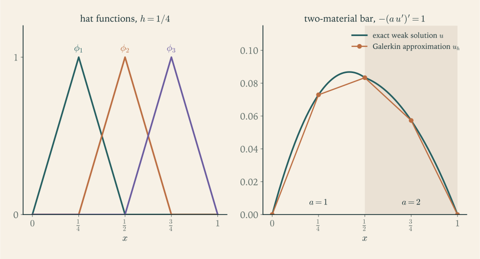
Figure 10.1 shows why the method is indifferent to the jump in the coefficient. Nothing in the assembly of \(K\) and \(F\) differentiates \(a\) ; the interface is handled by the weights on the mesh intervals. A finite difference approximation of the classical equation would have had to treat the interface as a special case.
Example 10.4: Galerkin with polynomials
The subspace need not consist of hat functions. Solve \(-u''+u=x\) on \((0,1)\) with zero boundary values; here \(a(u,v)=\int_0^1(u'v'+uv)\,dx\) is the \(H^1\) inner product and the exact solution is \(u=x-\sinh x/\sinh1\) , with \(u(\tfrac12)\approx0.0566\) and energy norm \(\lVert u\rVert_a\approx0.1425\) .
One function. With \(V_h\) spanned by \(\phi_1=x(1-x)\) : \(a(\phi_1,\phi_1)=\int_0^1(1-2x)^2dx+\int_0^1x^2(1-x)^2dx=\tfrac13+\tfrac1{30}=\tfrac{11}{30}\) and \(\ell(\phi_1)=\int_0^1x^2(1-x)\,dx=\tfrac1{12}\) , so \(c_1=\tfrac1{12}\cdot\tfrac{30}{11}=\tfrac5{22}\) and \(u_h(\tfrac12)=\tfrac5{88}\approx0.0568\) . The energy error is \(0.0369\) , about a quarter of \(\lVert u\rVert_a\) .
Two functions. Adding \(\phi_2=x^2(1-x)\) gives
and the energy error falls to \(0.0014\) , one percent of \(\lVert u\rVert_a\) . The midpoint value is again \(\tfrac5{88}\) : the energy norm, which the method minimizes, has improved by a factor of twenty-five, while one particular point value has not moved. Galerkin’s method is optimal in the norm of Theorem 10.5 and makes no promise about any other measure of error.
10.4 Convergence
Céa’s lemma turns an approximation estimate into an error estimate. For hat functions the natural candidate \(v\in V_h\) is the piecewise linear interpolant \(I_hu\) , which agrees with \(u\) at the mesh points.
Lemma 10.7 (interpolation error on one mesh interval). Let \(w\in C^2[p,q]\) with \(q-p=h\) , and let \(I_hw\) be the linear function with the same values at \(p\) and \(q\) . Then
Proof. The difference \(e=w-I_hw\) vanishes at \(p\) and \(q\) , so by Rolle’s theorem \(e'(\xi)=0\) for some \(\xi\in(p,q)\) . Since \(I_hw\) is linear, \(e''=w''\) , and \(e'(x)=\int_\xi^xw''(s)\,ds\) . By the Cauchy–Schwarz inequality \(e'(x)^2\le h\int_p^q(w'')^2ds\) for every \(x\) , and integrating over the interval gives the claim.
Theorem 10.8 (first-order convergence). Let \(a\) and \(\ell\) satisfy the hypotheses of Theorem 10.2 on \(V=H_0^1(0,1)\) , let \(V_h\) be the space of hat functions for a mesh of width \(h\) , and suppose the solution \(u\) is \(C^2\) on each closed mesh interval. Then
Proof. The interpolant \(I_hu\) belongs to \(V_h\) , so by Céa’s lemma \(\lVert u-u_h\rVert_{H^1}\le\tfrac M\alpha\lVert u-I_hu\rVert_{H^1}\) . The function \(u-I_hu\) is in \(H_0^1(0,1)\) , where \(C_P=1/\pi\) , so \(\lVert u-I_hu\rVert_{H^1}^2\le(1+\pi^{-2})\lVert(u-I_hu)'\rVert^2\) . Summing Lemma 10.7 over the mesh intervals bounds the last norm by \(h\) times the square root of the sum.
Halving the mesh width halves the bound on the error in the energy norm. In Example 10.2, with \(M=\alpha=1\) in the energy norm and \(\int(u'')^2=1\) , the bound for \(\lVert(u-u_h)'\rVert\) is \(h=0.25\) against the true value \(0.0722\) : correct order, pessimistic constant. In Example 10.3 the solution is \(C^2\) on each mesh interval because the interface is a node, and the theorem applies; had the interface fallen inside a mesh interval, the kink in \(u\) would have reduced the rate.
In several dimensions the same construction, with triangles or tetrahedra in place of intervals and hat functions that are pyramids over the patches of elements around each node, is the finite element method. Theorems 10.2 and 10.5 apply without change. For the heat equation one applies Galerkin’s method in the space variables only, which replaces the partial differential equation by a system of ordinary differential equations for the coefficients \(c_j(t)\) . How to build meshes, solve the resulting large sparse systems, and control errors in other norms is the business of Numerical Analysis, which owns those methods.
Common mistake. Checking coercivity in the wrong space or the wrong norm. For the pure Neumann problem \(-\Delta u=f\) , \(\partial u/\partial\nu=0\) , the form \(a(u,v)=\int\nabla u\cdot\nabla v\,dx\) lives on \(V=H^1(\Omega)\) , and the tempting line “\(a(v,v)=\lVert\nabla v\rVert^2\) , so \(a\) is coercive” is false: coercivity requires a lower bound by the full norm \(\lVert v\rVert_{H^1}^2\) , and a nonzero constant has \(a(v,v)=0\) . The Poincaré inequality that rescued the Dirichlet problem holds on \(H_0^1\) , not on \(H^1\) . The failure is real, not technical: the Neumann problem has no solution unless \(\int_\Omega f\,dx=0\) , and then infinitely many (Exercise 4). Before invoking Lax–Milgram, write down the space, the norm, and the three inequalities, and for coercivity test the constants and the first eigenfunction.
10.5 Choosing a method
The book has developed five families of tools. They answer different questions, and a given problem usually calls for more than one. The following table summarizes what each needs and what it delivers.
| Method | Needs | Delivers | Stops working when |
|---|---|---|---|
| Characteristics (Chapter 2) | a first-order equation, or a factorization into first-order ones | the solution along explicit curves; breaking time; shock speeds | characteristics cross, unless shocks and an entropy rule are added |
| Fundamental solutions and kernels (Chapters 4, 5, 6) | constant coefficients; the whole space, a half-space, or a ball | an integral formula; smoothing, speed of propagation, decay | the region or the coefficients are general |
| Separation of variables and Fourier series (Chapter 7) | an interval, rectangle, or disc; homogeneous boundary conditions on coordinate lines | a series; decay rates and frequencies; best constants | the geometry does not separate |
| Maximum principle and energy (Chapters 3, 5, 6) | only the type of the equation and the signs in it | uniqueness, stability, bounds, comparison, finite speed | a formula or an existence proof is wanted |
| Weak formulation, Lax–Milgram, Galerkin (Chapters 9, 10) | a coercive bilinear form on a Hilbert space | existence, uniqueness, stability for general regions and rough data; a computable approximation with an error bound | coercivity fails; pointwise regularity is wanted without further work |
Three questions sort most problems. First, what is the type? It fixes which side conditions are admissible and which qualitative tools exist: a maximum principle for elliptic and parabolic equations, an energy identity and a finite speed for hyperbolic ones. Second, how special are the geometry and the coefficients? Whole space and constant coefficients invite a kernel; a rectangle invites separation; a general region leaves the weak formulation. Third, what is actually being asked? A bound, a rate, or a uniqueness statement rarely requires solving anything.
Example 10.5: Four problems, four choices
A pollutant in a river whose speed depends on concentration. The model is a scalar conservation law \(u_t+\phi(u)_x=0\) , first order. Use characteristics to find the solution up to the breaking time \(-1/\min F'\) of Theorem 2.5, and beyond it the Rankine–Hugoniot and entropy conditions. No other tool in the table applies to a nonlinear first-order equation.
How long until a heated slab is within one percent of the temperature of its faces. A parabolic problem on an interval with constant coefficients. The question is a rate, so separation of variables is the tool: by Theorem 7.10 the slowest mode decays like \(e^{-k\pi^2t/L^2}\) , giving a time of about \(\log(100)\,L^2/(\pi^2k)\) once the first mode dominates, as in Exercise 7.7. The maximum principle gives the same rate with explicit bounds if the initial profile lies between two multiples of the first eigenfunction, as in Example 5.3.
Whether a measured steady temperature field inside a region can exceed all boundary readings. An elliptic problem and a qualitative question. No solving is needed: the weak maximum principle, Theorem 3.6, says it cannot when there are no interior sources, and Theorem 3.8 bounds the excess when there are.
The deflection of a membrane of irregular outline, made of two materials, under a load. An elliptic problem on a general region with a discontinuous coefficient. No kernel or series is available, and there is not even a classical formulation at the interface. Put it in weak form, check uniform ellipticity to get existence and uniqueness from Theorem 10.4, and compute a Galerkin approximation on a mesh that follows the interface, as in Example 10.3. The maximum principle can still be used on the weak solution’s smooth pieces to sanity-check the computed values.
The classical and the weak theory are not rivals. The classical theory explains what solutions look like and why: averaging, smoothing, propagation, reflection. The weak theory guarantees that solutions exist in situations where no formula ever will, and it tells a computer how to find them. A working analyst uses the first to know what to expect and the second to be sure of it.
Exercises
-
Let \(K\) be a real \(N\times N\) matrix, not necessarily symmetric, with \(c^{\top}Kc\ge\alpha\lvert c\rvert^2\) for all \(c\in\mathbb R^N\) and some \(\alpha>0\) . Prove that \(K\) is invertible and that \(\lvert K^{-1}F\rvert\le\lvert F\rvert/\alpha\) . Check both statements for the matrix with rows \((1,2)\) and \((-2,1)\) .
Solution
Invertibility. If \(Kc=0\) then \(0=c^{\top}Kc\ge\alpha\lvert c\rvert^2\) , so \(c=0\) . The null space of \(K\) is trivial, and by the rank–nullity theorem a square matrix with trivial null space has full rank, so it is invertible.
The bound. Let \(c=K^{-1}F\) . Then \(\alpha\lvert c\rvert^2\le c^{\top}Kc=c^{\top}F\le\lvert c\rvert\,\lvert F\rvert\) by the Cauchy–Schwarz inequality, and dividing by \(\lvert c\rvert\) when it is not zero gives \(\lvert c\rvert\le\lvert F\rvert/\alpha\) .
The example. For \(K\) with rows \((1,2)\) and \((-2,1)\) , \(c^{\top}Kc=c_1^2+2c_1c_2-2c_1c_2+c_2^2=\lvert c\rvert^2\) , so the hypothesis holds with \(\alpha=1\) although \(K\) is not symmetric: only the symmetric part of a matrix contributes to \(c^{\top}Kc\) . The determinant is \(1+4=5\) , the inverse has rows \(\tfrac15(1,-2)\) and \(\tfrac15(2,1)\) , and \(\lvert K^{-1}F\rvert^2=\tfrac1{25}\bigl((F_1-2F_2)^2+(2F_1+F_2)^2\bigr)=\tfrac15\lvert F\rvert^2\) . So \(\lvert K^{-1}F\rvert=\lvert F\rvert/\sqrt5\le\lvert F\rvert\) , as predicted. This is Theorem 10.2 in finite dimensions, with the existence half supplied by counting dimensions.
-
Verify the hypotheses of the Lax–Milgram theorem for the problem of Example 9.4 generalized to a load: find \(u\in H^1(0,1)\) with \(\int_0^1(u'v'+uv)\,dx=\int_0^1fv\,dx+\gamma v(1)\) for all \(v\in H^1(0,1)\) , where \(f\in L^2(0,1)\) . Give \(M\) , \(\alpha\) , and a bound for \(\lVert\ell\rVert_{V'}\) .
Answer
\(V=H^1(0,1)\) and \(a\) is the \(H^1\) inner product, so \(M=1\) and \(\alpha=1\) . For the functional, \(\lvert\int_0^1fv\,dx\rvert\le\lVert f\rVert\,\lVert v\rVert_{H^1}\) , and by Theorem 9.3, \(\lvert v(1)\rvert\le\lVert v\rVert+\lVert v'\rVert\le\sqrt2\,\lVert v\rVert_{H^1}\) . So \(\lVert\ell\rVert_{V'}\le\lVert f\rVert+\sqrt2\,\lvert\gamma\rvert\) , and there is exactly one solution, with \(\lVert u\rVert_{H^1}\le\lVert f\rVert+\sqrt2\lvert\gamma\rvert\) .
-
Let \(c\) be a bounded measurable function on a bounded open set \(\Omega\) with \(c(x)\ge c_0>0\) . Show that \(a(u,v)=\int_\Omega(\nabla u\cdot\nabla v+c\,uv)\,dx\) is bounded and coercive on \(H^1(\Omega)\) , and state the boundary value problem that the resulting weak solution solves when it is smooth.
Hint
\(\lvert a(u,v)\rvert\le\max(1,\sup c)\,\lVert u\rVert_{H^1}\lVert v\rVert_{H^1}\) and \(a(v,v)\ge\min(1,c_0)\,\lVert v\rVert_{H^1}^2\) ; no Poincaré inequality is needed because the zeroth-order term controls \(\lVert v\rVert\) . The problem is \(-\Delta u+cu=f\) with the natural condition \(\partial u/\partial\nu=0\) .
-
For the pure Neumann problem \(-u''=f\) on \((0,1)\) with \(u'(0)=u'(1)=0\) , write the weak form on \(H^1(0,1)\) , show that a solution can exist only if \(\int_0^1f\,dx=0\) , and prove that under this condition there is exactly one weak solution with \(\int_0^1u\,dx=0\) , by applying the Lax–Milgram theorem on the subspace of functions with mean zero.
Solution
Weak form. Multiplying by \(v\in H^1(0,1)\) and integrating by parts, the boundary terms vanish by the Neumann conditions: find \(u\in H^1(0,1)\) with \(\int_0^1u'v'\,dx=\int_0^1fv\,dx\) for all \(v\in H^1(0,1)\) .
Necessary condition. The constant \(v=1\) is an admissible test function. It gives \(0=\int_0^1f\,dx\) . So no solution exists unless \(f\) has mean zero. And if \(u\) is a solution so is \(u+C\) , so the form cannot be coercive on \(H^1(0,1)\) ; indeed \(a(1,1)=0\) .
Existence on the mean-zero subspace. Let \(W=\{v\in H^1(0,1):\int_0^1v\,dx=0\}\) . It is the null space of the bounded linear functional \(v\mapsto\int_0^1v\,dx\) , hence a closed subspace of \(H^1(0,1)\) and a Hilbert space. On \(W\) , Exercise 9.8 gives \(\lVert v\rVert\le\lVert v'\rVert\) , so \(a(v,v)=\lVert v'\rVert^2\ge\tfrac12\lVert v\rVert_{H^1}^2\) : coercive with \(\alpha=\tfrac12\) . The form is bounded with \(M=1\) , and \(\ell(v)=\int fv\,dx\) is bounded. By Theorem 10.2 there is exactly one \(u\in W\) with \(a(u,w)=\ell(w)\) for all \(w\in W\) .
Back to all test functions. An arbitrary \(v\in H^1(0,1)\) is \(w+m\) with \(m\) its mean and \(w\in W\) . Then \(a(u,v)=a(u,w)=\ell(w)=\ell(v)-m\int_0^1f\,dx=\ell(v)\) , using the compatibility condition. So \(u\) solves the original weak problem, and it is the only solution with mean zero, since two solutions in \(W\) differ by an element of \(W\) with zero energy. The compatibility condition and the normalization are the two requirements found for the classical problem in Exercise 1.18.
-
For constant \(b\) consider \(-u''+bu'=f\) on \((0,1)\) with \(u(0)=u(1)=0\) . Show that \(\int_0^1v'v\,dx=0\) for \(v\in H_0^1(0,1)\) , deduce that the bilinear form is coercive for every \(b\) , and compare with the sufficient condition of Theorem 10.4.
Solution
For a test function \(v\) , \(\int_0^1v'v\,dx=\tfrac12\int_0^1(v^2)'\,dx=\tfrac12[v^2]_0^1=0\) . Both sides of \(\int_0^1v'v\,dx=0\) are continuous in the \(H^1\) norm, so the identity extends to \(v\in H_0^1(0,1)\) by density; alternatively use Exercise 9.3. The bilinear form is \(a(u,v)=\int_0^1u'v'\,dx+b\int_0^1u'v\,dx\) , and therefore
\[ a(v,v)=\lVert v'\rVert^2+b\cdot0=\lVert v'\rVert^2\ge\frac{1}{1+\pi^{-2}}\lVert v\rVert_{H^1}^2 \]for every real \(b\) . The form is bounded, with \(M\le1+\lvert b\rvert\) , so by Theorem 10.2 the problem has a unique weak solution for every \(b\) and every \(f\in L^2(0,1)\) .
Theorem 10.4 guarantees coercivity only when \(\beta C_P<\theta\) , here \(\lvert b\rvert<\pi\) . That condition treats the transport term as a perturbation and estimates it by its size. The present argument uses its structure: a constant transport field moves the quantity without creating or destroying energy, so the term is exactly skew and contributes nothing to \(a(v,v)\) . The price of large \(b\) appears elsewhere: \(M\) grows with \(\lvert b\rvert\) while \(\alpha\) does not, so the constant \(M/\alpha\) in Céa’s lemma deteriorates (Exercise 10.16).
-
A student writes: “For the Neumann problem \(-\Delta u=f\) in \(\Omega\) , \(\partial u/\partial\nu=0\) , the form \(a(u,v)=\int\nabla u\cdot\nabla v\,dx\) satisfies \(a(v,v)=\lVert\nabla v\rVert^2\ge0\) , so it is coercive, and by Lax–Milgram there is a unique solution for every \(f\in L^2(\Omega)\) .” Identify the false step, and show by a direct argument that both the existence and the uniqueness claimed are false.
Solution
The false step is “\(a(v,v)=\lVert\nabla v\rVert^2\ge0\) , so it is coercive”. Coercivity on \(V=H^1(\Omega)\) means \(a(v,v)\ge\alpha\lVert v\rVert_{H^1}^2=\alpha(\lVert v\rVert^2+\lVert\nabla v\rVert^2)\) with \(\alpha>0\) . For the constant function \(v=1\) the left side is \(0\) and the right side is \(\alpha\lvert\Omega\rvert>0\) . Nonnegativity is not coercivity, and the Poincaré inequality that would bridge the gap is available on \(H_0^1(\Omega)\) only.
Uniqueness fails. If \(u\) satisfies \(\int\nabla u\cdot\nabla v\,dx=\int fv\,dx\) for all \(v\in H^1(\Omega)\) , so does \(u+C\) for every constant \(C\) , because \(\nabla C=0\) .
Existence fails. Test with \(v=1\) : the left side is zero, so a solution requires \(\int_\Omega f\,dx=0\) . For \(f=1\) , say, there is no solution. Physically, a body insulated all round with a net heat source cannot have a steady temperature.
The correct statement, as in Exercise 10.4: if \(\int_\Omega f\,dx=0\) , there is exactly one weak solution with mean zero, obtained by applying Lax–Milgram on the closed subspace of mean-zero functions, where a Poincaré inequality for mean-zero functions restores coercivity.
-
For which real \(\lambda\) is the form \(\int_0^1u'v'\,dx-\lambda\int_0^1uv\,dx\) coercive on \(H_0^1(0,1)\) ? For \(\lambda=4\pi^2\) find a nonzero solution of the homogeneous problem and the condition on \(f\) that is necessary for the inhomogeneous problem to have a solution.
Answer
Coercive exactly for \(\lambda<\pi^2\) : for \(\lambda\ge\pi^2\) , \(a_\lambda(\sin\pi x,\sin\pi x)=\tfrac12(\pi^2-\lambda)\le0\) . For \(\lambda=4\pi^2\) the function \(\sin(2\pi x)\) solves the homogeneous problem, and testing with it shows that a solution of the inhomogeneous problem requires \(\int_0^1f\sin(2\pi x)\,dx=0\) .
-
Assemble and solve the Galerkin system for \(-u''=x\) on \((0,1)\) , \(u(0)=u(1)=0\) , with hat functions on the mesh of width \(h=\tfrac13\) . Compare the nodal values with the exact solution.
Solution
With \(h=\tfrac13\) the interior nodes are \(x_1=\tfrac13\) and \(x_2=\tfrac23\) . The stiffness matrix is \(K=\tfrac1h\begin{pmatrix}2&-1\\-1&2\end{pmatrix}=\begin{pmatrix}6&-3\\-3&6\end{pmatrix}\) . For the load, \(F_i=\int_0^1x\,\phi_i\,dx\) ; since \(x=x_i+(x-x_i)\) and \(\phi_i\) is symmetric about \(x_i\) with integral \(h\) , \(F_i=hx_i\) , so \(F=(\tfrac19,\tfrac29)\) . The system is
\[ 6c_1-3c_2=\tfrac19,\qquad-3c_1+6c_2=\tfrac29 . \]Adding twice the first equation to the second gives \(9c_1=\tfrac49\) , so \(c_1=\tfrac4{81}\) , and then \(c_2=2c_1-\tfrac1{27}=\tfrac5{81}\) .
The exact solution of \(-u''=x\) with zero boundary values is \(u=\tfrac16x(1-x^2)\) , as in Example 4.2. Its nodal values are \(u(\tfrac13)=\tfrac16\cdot\tfrac13\cdot\tfrac89=\tfrac4{81}\) and \(u(\tfrac23)=\tfrac16\cdot\tfrac23\cdot\tfrac59=\tfrac5{81}\) . The Galerkin values agree exactly, as Proposition 10.6 predicts, although the mesh is coarse and the load is not constant. Between the nodes \(u_h\) is the linear interpolant of \(u\) .
-
Apply Galerkin’s method with a single hat function, \(h=\tfrac12\) , to \(-u''+u=1\) on \((0,1)\) with zero boundary values. Compare \(u_h(\tfrac12)\) with the exact value and explain, using the proof of Proposition 10.6, why the nodal value is not exact here.
Answer
\(a(\phi,\phi)=\int_0^1(\phi')^2dx+\int_0^1\phi^2dx=4+\tfrac13=\tfrac{13}{3}\) and \(\ell(\phi)=\tfrac12\) , so \(u_h(\tfrac12)=\tfrac3{26}\approx0.1154\) . The exact solution \(u=1-\cosh(x-\tfrac12)/\cosh\tfrac12\) has \(u(\tfrac12)\approx0.1132\) . The function \(w\) with \(a(v,w)=v(\tfrac12)\) for all \(v\) now solves \(-w''+w=\delta_{1/2}\) and is built from hyperbolic functions, not straight lines, so it is not in \(V_h\) and the argument of Proposition 10.6 fails.
-
In Example 10.2 verify the identity \(\lVert u-u_h\rVert_a^2=\lVert u\rVert_a^2-\lVert u_h\rVert_a^2\) by computing the left side directly on one mesh interval, and predict the energy error for \(h=\tfrac18\) .
Answer
On one interval, \(u'-u_h'\) is linear with slope \(-1\) and mean zero, so \(\int(u'-u_h')^2dx=\int_{-h/2}^{h/2}s^2ds=h^3/12\) ; four intervals give \(\tfrac{h^2}{12}=\tfrac1{192}\) for \(h=\tfrac14\) , matching \(\tfrac1{12}-\tfrac5{64}\) . For \(h=\tfrac18\) the energy error is \(h/\sqrt{12}\approx0.0361\) , half as large.
-
For \(-u''=f\) on \((0,1)\) with \(f\) continuous and hat functions of width \(h\) , show that \(\lVert(u-u_h)'\rVert\le h\lVert f\rVert\) . For \(f=1\) compare this bound with the exact error for \(h=\tfrac14\) and for general \(h\) .
Hint
By Theorem 10.5(d), \(\lVert(u-u_h)'\rVert\le\lVert(u-I_hu)'\rVert\) ; by Lemma 10.7 summed over the intervals this is at most \(h\lVert u''\rVert=h\lVert f\rVert\) . For \(f=1\) the exact error is \(h/\sqrt{12}\approx0.289\,h\) .
-
Apply Galerkin’s method to \(-u''=f\) on \((0,1)\) with zero boundary values, using the subspace spanned by \(\sin(n\pi x)\) for \(n=1,\dots,N\) . Show that \(K\) is diagonal, find \(u_N\) in terms of the sine coefficients of \(f\) , and identify it with a partial sum of the series solution of Chapter 7.
Solution
Let \(\phi_n=\sin(n\pi x)\) . Then \(\phi_n'=n\pi\cos(n\pi x)\) and, by the orthogonality of the cosines,
\[ K_{mn}=\int_0^1\phi_n'\phi_m'\,dx=mn\pi^2\int_0^1\cos(n\pi x)\cos(m\pi x)\,dx=\frac{n^2\pi^2}{2}\ \text{ if }m=n,\quad 0\ \text{ otherwise}. \]So \(K\) is diagonal. The load vector is \(F_n=\int_0^1f\sin(n\pi x)\,dx=\tfrac12f_n\) , where \(f_n=2\int_0^1f\sin(n\pi x)\,dx\) are the sine coefficients of \(f\) . The system \(Kc=F\) decouples: \(c_n=f_n/(n^2\pi^2)\) , and
\[ u_N(x)=\sum_{n=1}^N\frac{f_n}{n^2\pi^2}\,\sin(n\pi x). \]This is the \(N\) -th partial sum of the series obtained by separation of variables: expanding \(u=\sum b_n\sin(n\pi x)\) in \(-u''=f\) gives \(n^2\pi^2b_n=f_n\) . So the Fourier method of Chapter 7 is Galerkin’s method with eigenfunctions as basis. The eigenfunctions are exactly the basis that diagonalizes the stiffness matrix, which is why no linear system had to be solved in Chapter 7; the hat functions give instead a sparse, tridiagonal matrix on any mesh, which is the property that survives on regions where eigenfunctions are unknown.
-
Use Céa’s lemma and Theorem 7.8 to prove that the Galerkin approximations of Exercise 12 converge to the weak solution in \(H^1\) as \(N\to\infty\) , for every \(f\in L^2(0,1)\) .
Hint
By Theorem 10.5(c) with \(M=1\) and \(\alpha=1/(1+\pi^{-2})\) it suffices to show that the partial sums \(S_Nu\) of the sine series of \(u\) converge to \(u\) in \(H^1\) . As in Corollary 7.9, \((S_Nu)'\) is the \(N\) -th partial sum of the cosine series of \(u'\in L^2(0,1)\) , which converges to \(u'\) in mean square by the cosine version of Theorem 7.8; and \(S_Nu\to u\) in \(L^2\) by Theorem 7.8 itself.
-
For each problem name the method you would use first and what it would deliver: (a) \(u_t+3u_x=e^{-t}\) on the line; (b) the steady temperature in a disc with prescribed boundary temperature; (c) a bound for \(\max\lvert u\rvert\) when \(-\Delta u=f\) in an irregular region with \(u=0\) on the boundary; (d) the frequencies of a vibrating string; (e) existence of a steady temperature in an L-shaped plate with a heat source in \(L^2\) ; (f) the time at which a wave released at the origin first reaches a given point.
Answer
(a) Characteristics with a source: \(u=g(x-3t)+1-e^{-t}\) . (b) Poisson’s formula for the disc, or separation in polar coordinates; an explicit solution. (c) The maximum principle with a barrier, Theorem 3.8: a bound without solving. (d) Separation of variables: frequencies \(nc/(2L)\) . (e) Weak formulation and Lax–Milgram, Theorem 10.3: existence and uniqueness in \(H_0^1\) , with no claim of smoothness at the corner. (f) Domain of dependence, Section 6.3 or Theorem 6.6: the distance divided by \(c\) .
-
Compare the four well-posedness statements Theorem 3.7, Theorem 5.5, Theorem 6.2, and Theorem 10.3 by naming for each the class of data, the class of solutions, and the norm in which continuous dependence holds. Which of the four also proves existence?
Hint
Theorem 3.7: continuous boundary data, solutions in \(C^2(\Omega)\cap C(\overline\Omega)\) , maximum norm; no existence. Theorem 5.5: continuous initial and boundary data, classical solutions on the rectangle, maximum norm; no existence. Theorem 6.2: \(g\in C^2\) , \(h\in C^1\) , solutions in \(C^2\) , maximum norm on bounded time intervals; existence by formula. Theorem 10.3: \(f\in L^2\) , solutions in \(H_0^1\) , \(H^1\) norm; existence by Lax–Milgram.
-
Apply Galerkin’s method with a single hat function, \(h=\tfrac12\) , to \(-u''+10u'=1\) on \((0,1)\) with zero boundary values. Find \(u_h(\tfrac12)\) , compare it with the exact value, and explain the poor result in terms of the constant in Céa’s lemma.
Solution
With the single hat \(\phi\) centred at \(\tfrac12\) : \(\int_0^1(\phi')^2dx=4\) , and \(\int_0^1\phi'\phi\,dx=0\) by Exercise 10.5, so \(a(\phi,\phi)=4+10\cdot0=4\) . The load is \(\ell(\phi)=\int_0^1\phi\,dx=\tfrac12\) . Hence \(u_h(\tfrac12)=c=\tfrac18=0.125\) , the same value as for the problem without transport: one symmetric basis function cannot see the transport term at all.
The exact solution: a particular solution of \(-u''+10u'=1\) is \(x/10\) , the homogeneous solutions are \(1\) and \(e^{10x}\) , and the boundary conditions give
\[ u(x)=\frac{x}{10}-\frac{e^{10x}-1}{10\,(e^{10}-1)},\qquad u(\tfrac12)=0.05-\frac{e^{5}-1}{10\,(e^{10}-1)}\approx0.0493 . \]The Galerkin value is more than twice too large.
Céa’s lemma explains this in two ways. In the norm \(\lVert v'\rVert\) the form has \(\alpha=1\) and \(M\) of the order \(1+10\,C_P=1+10/\pi\approx4.2\) , so the Galerkin error may be about four times the best approximation error. And the best approximation error is itself large: the exact solution follows the line \(x/10\) across most of the interval and then drops to zero in a boundary layer of width about \(0.1\) near \(x=1\) , which no multiple of a single hat of width \(1\) can imitate. Both factors improve as \(h\) decreases below the layer width. Coercivity guarantees a solution and a convergent method; it does not guarantee a good answer on a coarse mesh.
-
Let \(g\) be a function in \(H^1(\Omega)\) and \(f\in L^2(\Omega)\) on a bounded open set. Show how to obtain a function \(u\in H^1(\Omega)\) with \(u-g\in H_0^1(\Omega)\) and \(\int\nabla u\cdot\nabla v\,dx=\int fv\,dx\) for all \(v\in H_0^1(\Omega)\) from Theorem 10.2, and state the estimate it gives.
Hint
Put \(u=g+w\) and seek \(w\in H_0^1(\Omega)\) with \(\int\nabla w\cdot\nabla v\,dx=\int fv\,dx-\int\nabla g\cdot\nabla v\,dx\) for all \(v\in H_0^1(\Omega)\) . The right side is a bounded functional with norm at most \(\lVert f\rVert+\lVert\nabla g\rVert\) , so Theorem 10.2 gives a unique \(w\) with \(\lVert w\rVert_{H^1}\le(1+C_P^2)\bigl(\lVert f\rVert+\lVert\nabla g\rVert\bigr)\) .