A disease affects one person in a hundred. A screening test detects it in \(90\) percent of those who have it, and gives a false alarm in \(5\) percent of those who do not. A person chosen at random from the population tests positive. How likely is it that the person has the disease?

Asked this question, most people, including many physicians in published surveys, answer something near \(90\) percent. The correct answer is about \(15\) percent. The gap is not a matter of arithmetic. It comes from confusing two different conditional probabilities: the probability of a positive test given the disease, which is \(0.90\) and is a property of the test, and the probability of the disease given a positive test, which also depends on how rare the disease is. This chapter defines conditional probability, derives the two rules that connect a conditional probability to its reverse, and introduces independence, the situation in which conditioning changes nothing.

2.1 Conditioning as a change of sample space

Suppose we learn that an event \(B\) has occurred. Outcomes outside \(B\) are no longer possible, and the outcomes inside \(B\) should keep their relative weights, since we have learned nothing that distinguishes among them. Rescaling so that the total is again one leads to the definition.

When outcomes are equally likely this is a ratio of counts, \(\lvert A\cap B\rvert/\lvert B\rvert\) : among the outcomes in which \(B\) occurs, the fraction in which \(A\) occurs as well. In the frequency interpretation it is the long-run fraction of the occurrences of \(B\) that are also occurrences of \(A\) . The condition \(P(B)>0\) is needed for the quotient to make sense; conditioning on events of probability zero, such as a continuous measurement taking an exact value, requires the density methods of Chapter 5.

The proposition has a practical meaning: every rule proved in Chapter 1 holds for conditional probabilities with the same condition throughout. For instance \(P(A^c\mid B)=1-P(A\mid B)\) . What is not allowed is to complement the condition: \(P(A\mid B^c)\) is a different quantity with no fixed relation to \(P(A\mid B)\) .

2.2 The multiplication rule

Definition 2.1 can be read backwards: \(P(A\cap B)=P(B)\,P(A\mid B)\) . In this form it computes the probability that two things both happen from the probability of the first and the conditional probability of the second, which is how sequential experiments are naturally described. The rule extends to any number of stages.

A probability tree is a picture of this theorem. Each branch from a node carries the conditional probability of the next event given the path so far; the probability of a path from the root to a leaf is the product of the numbers along it; and the branches leaving any node have probabilities that sum to one, by Proposition 2.2.

2.3 Total probability and Bayes’ rule

Often the probability of an event is known only case by case. The law of total probability assembles the cases.

The formula is a weighted average: the conditional probabilities \(P(A\mid B_i)\) are averaged with weights \(P(B_i)\) . Consequently \(P(A)\) always lies between the smallest and the largest of the \(P(A\mid B_i)\) . A simple instance: what is the probability that the second card dealt from a deck is an ace? Condition on whether the first card is an ace:

the same as for the first card, as symmetry demands. A card that has been dealt but not seen carries no information.

The proof is two lines, and the theorem is nevertheless one of the most consequential in the subject, because of how its ingredients arise in practice. The \(B_i\) are competing explanations, or hypotheses. The numbers \(P(B_i)\) , called prior probabilities, describe the situation before the evidence \(A\) is seen. The numbers \(P(A\mid B_i)\) , the likelihoods, say how probable the evidence is under each explanation, and they are usually what a model supplies directly: they run in the causal direction, from explanation to evidence. Bayes’ rule turns them around into the posterior probabilities \(P(B_i\mid A)\) , which run from evidence to explanation and are what one wants to know.

Example 2.3: The screening test

Let \(D\) be the event that the person has the disease and \(T\) the event that the test is positive. The data are \(P(D)=0.01\) , \(P(T\mid D)=0.90\) , and \(P(T\mid D^c)=0.05\) . The partition is \(\{D,D^c\}\) .

By the law of total probability,

\[ P(T)=0.90\cdot 0.01+0.05\cdot 0.99=0.009+0.0495=0.0585, \]

and by Bayes’ rule

\[ P(D\mid T)=\frac{0.009}{0.0585}=\frac{2}{13}\approx 0.154 . \]

The same computation in whole numbers is easier to believe. Of \(10{,}000\) people, \(100\) have the disease and \(9{,}900\) do not. The test is positive for \(90\) of the \(100\) and for \(495\) of the \(9{,}900\) . So \(585\) people test positive, of whom only \(90\) are ill, and \(90/585=2/13\) . The false positives are a small fraction of a very large group, and they outnumber the true positives, which are a large fraction of a very small one.

A negative result, on the other hand, is highly informative here: \(P(D\mid T^c)=\dfrac{0.10\cdot 0.01}{0.10\cdot 0.01+0.95\cdot 0.99}=\dfrac{2}{1883}\approx 0.0011\) , about one in a thousand.

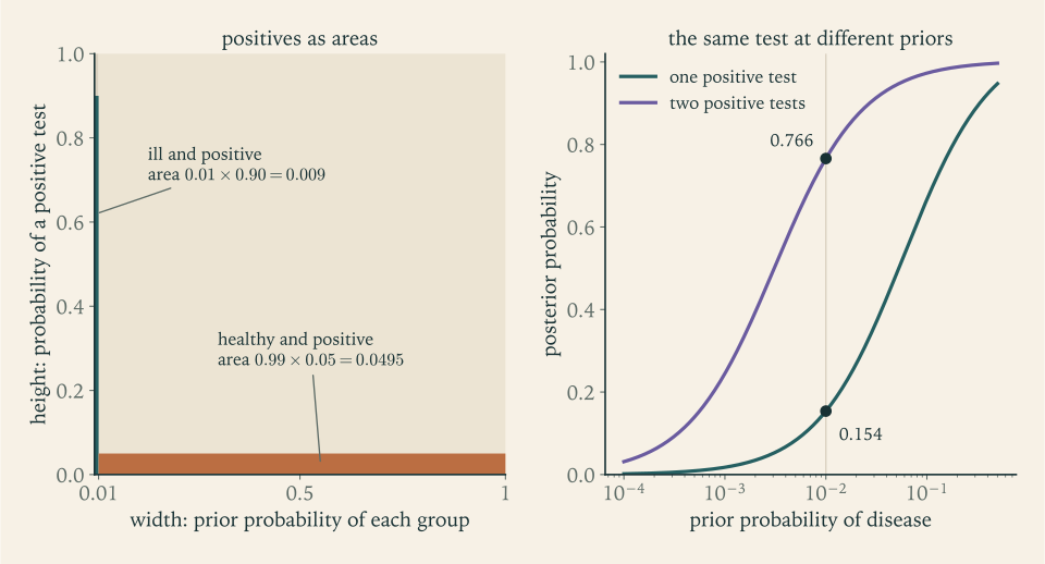
In the left panel of Figure 2.1 the widths of the columns are the prior probabilities and the shaded heights are the likelihoods, so each shaded area is a product \(P(T\mid B_i)P(B_i)\) . Conditioning on a positive test discards everything unshaded, and the posterior probability of disease is the sliver’s share of the total shaded area. The right panel answers the question that the opening numbers leave hanging: how can a good test give such a weak conclusion? The test is the same along each curve; only the prior changes. At a prior of \(0.10\) , as in a clinic where patients already have symptoms, the same positive result gives a posterior of \(2/3\) .

Common mistake. Reversing a conditional probability. The statements “\(90\) percent of ill people test positive” and “\(90\) percent of people who test positive are ill” have the same words in a different order, and the second does not follow from the first. In symbols, \(P(T\mid D)\) and \(P(D\mid T)\) differ by the factor \(P(D)/P(T)\) , which here is \(0.01/0.0585\approx 0.17\) . The same reversal appears in court as the claim that because a match would be unlikely if the defendant were innocent, the defendant is unlikely to be innocent given a match. The repair is always the same: write the prior, write both likelihoods, and compute the denominator by total probability before stating any posterior.

There is a form of Bayes’ rule for two hypotheses that makes repeated updating almost mechanical. The odds of an event \(B\) are \(P(B)/P(B^c)\) ; odds of \(1\) to \(99\) correspond to probability \(1/100\) , and odds \(o\) correspond to probability \(o/(1+o)\) .

Proposition 2.7 (Bayes’ rule in odds form). If \(0<P(B)<1\) and \(P(A)>0\) , then

\[ \frac{P(B\mid A)}{P(B^c\mid A)}=\frac{P(B)}{P(B^c)}\cdot\frac{P(A\mid B)}{P(A\mid B^c)}, \]

provided \(P(A\mid B^c)>0\) . In words: posterior odds equal prior odds times the likelihood ratio.

Proof. Write Bayes’ rule for \(B\) and for \(B^c\) . The two expressions have the same denominator \(P(A)\) , which cancels in the quotient.

For the screening test the likelihood ratio of a positive result is \(0.90/0.05=18\) . The prior odds are \(1/99\) , so the posterior odds are \(18/99=2/11\) , and the posterior probability is \(\frac{2/11}{1+2/11}=\frac{2}{13}\) , as before. A positive result multiplies the odds of disease by \(18\) ; it cannot do more, and eighteen times a very small number is still small.

2.4 Independence

Sometimes learning that \(B\) occurred does not change the probability of \(A\) at all: \(P(A\mid B)=P(A)\) . Multiplying out gives a condition that is symmetric in the two events and makes sense even when one of them has probability zero.

Independence is a property of the probability measure, not of the events as sets. It can be an assumption built into a model, as when we say that successive rolls of a die do not influence one another and therefore assign probability \(1/36\) to each ordered pair. Or it can be a conclusion, checked by computing both sides of the product rule. In the first role it is the most powerful simplifying assumption in probability; in the second it sometimes holds for no visible reason. On one roll of a fair die the events “even” and “at most four” are independent, since \(P(\{2,4\})=\tfrac13=\tfrac12\cdot\tfrac23\) , although both are statements about the same roll.

The same holds for mutually independent families: replacing any of the events by their complements leaves the family mutually independent. It is enough to show this when a single event, say \(A_1\) , is replaced, since the replacement can then be repeated one event at a time. A subcollection that does not contain \(A_1^c\) is unaffected. For one that does, let \(B\) be the intersection of its other members, which belong to the original family; then \(P(A_1^c\cap B)=P(B)-P(A_1\cap B)=P(B)-P(A_1)P(B)=P(A_1^c)\,P(B)\) , and \(P(B)\) is the product of the probabilities of its members. This is what justifies the most frequently used formula for independent trials. If each of \(n\) mutually independent trials succeeds with probability \(p\) , the events “trial \(k\) fails” are mutually independent with probability \(1-p\) each, so

Chapter 1 obtained this by counting in the case of dice. Independence delivers it for any \(p\) , whether or not there are equally likely outcomes behind it. A related application is the reliability of systems. If components work independently, a series system, which needs all of its components, works with the product of their probabilities, and a parallel system, which needs at least one, fails with the product of their failure probabilities. Two components in series, backed up in parallel by a third, each working with probability \(0.9\) , form a system that works with probability \(1-(1-0.9^2)(1-0.9)=0.981\) .

Why does the definition of mutual independence demand the product rule for every subcollection, and not just for pairs?

2.5 Solving problems by conditioning

Many problems that look intractable become short once the right partition is found. The partition is usually “what happened first” or “which hidden state holds”.

Exercises

1. Two fair dice are rolled. Find the conditional probability that the sum is eight given that the first die is even, that at least one die shows a six given that the sum is at least ten, and that both show a six given that at least one does. Then, for the family of Example 2.1, enlarge the sample space to include which child is met, each equally likely, and compute the probability of two boys given that the child met is a boy.

   Answer

   Sum eight given first die even: the \(18\) outcomes with an even first die include \((2,6)\) , \((4,4)\) , \((6,2)\) , so \(3/18=1/6\) . At least one six given sum at least ten: the six outcomes \((4,6),(5,5),(5,6),(6,4),(6,5),(6,6)\) include five with a six, so \(5/6\) . Both six given at least one six: \(1/11\) . For the family, the sample space has eight equally likely outcomes (family, child met); the child met is a boy in four of them, and in two of those the family is BB, so the probability is \(\tfrac12\) .

2. Prove the conditional form of the law of total probability: if \(B_1,\dots,B_n\) partition \(\Omega\) and \(P(B_i\cap C)>0\) for every \(i\) , then \(P(A\mid C)=\sum_i P(A\mid B_i\cap C)\,P(B_i\mid C)\) .

   Hint

   Work under the probability measure \(Q(\cdot)=P(\cdot\mid C)\) , which is legitimate by Proposition 2.2, and apply Theorem 2.5 to \(Q\) . Then check from Definition 2.1 that \(Q(A\mid B_i)=P(A\cap B_i\cap C)/P(B_i\cap C)=P(A\mid B_i\cap C)\) .

3. An urn holds five red balls and three blue balls, and three balls are drawn in order without replacement. Find the probability of the sequence red, blue, red; the probability that the second ball is red; and the conditional probability that the first ball was red given that the second is red.

   Solution

   Let \(R_k\) be the event that the \(k\) -th ball drawn is red. By the multiplication rule, following the composition of the urn as balls are removed,

   \[ P(R_1\cap R_2^c\cap R_3)=\frac58\cdot\frac37\cdot\frac46=\frac{5}{28}. \]

   For the second ball, condition on the first:

   \[ P(R_2)=P(R_2\mid R_1)P(R_1)+P(R_2\mid R_1^c)P(R_1^c)=\frac47\cdot\frac58+\frac57\cdot\frac38=\frac{35}{56}=\frac58 . \]

   This equals \(P(R_1)\) , as symmetry requires: every ball is equally likely to occupy the second position. Finally, by Bayes’ rule,

   \[ P(R_1\mid R_2)=\frac{P(R_2\mid R_1)P(R_1)}{P(R_2)}=\frac{(4/7)(5/8)}{5/8}=\frac47 . \]

   Notice that \(P(R_1\mid R_2)=P(R_2\mid R_1)\) . Conditioning on a later draw is as legitimate as conditioning on an earlier one; time order plays no role in the definition, only in how the model was specified.

4. Forty percent of incoming messages are spam. A certain word appears in \(25\) percent of spam messages and in \(1\) percent of other messages. Find the probability that a message containing the word is spam, and the probability that a message not containing it is spam.

   Solution

   Let \(S\) be the event that a message is spam and \(W\) the event that it contains the word. Then \(P(S)=0.4\) , \(P(W\mid S)=0.25\) , \(P(W\mid S^c)=0.01\) . Total probability gives \(P(W)=0.25\cdot 0.4+0.01\cdot 0.6=0.1+0.006=0.106\) , and Bayes’ rule gives

   \[ P(S\mid W)=\frac{0.1}{0.106}=\frac{50}{53}\approx 0.943 . \]

   For a message without the word, \(P(W^c\mid S)=0.75\) and \(P(W^c\mid S^c)=0.99\) , so

   \[ P(S\mid W^c)=\frac{0.75\cdot 0.4}{0.75\cdot 0.4+0.99\cdot 0.6}=\frac{0.3}{0.894}=\frac{50}{149}\approx 0.336 . \]

   The word is strong evidence when present, with likelihood ratio \(25\) , and weak evidence when absent, with likelihood ratio \(0.75/0.99\approx 0.76\) , so its absence lowers the probability of spam only from \(0.4\) to about \(0.34\) .

5. For the test of Example 2.3, find the posterior probability of disease after a positive result when the prior probability is \(0.10\) in place of \(0.01\) , and find the probability of disease after a negative result at the original prior, giving both as fractions.

   Answer

   At prior \(0.10\) : \(\dfrac{0.9\cdot 0.1}{0.9\cdot 0.1+0.05\cdot 0.9}=\dfrac{0.09}{0.135}=\dfrac23\) . After a negative result at prior \(0.01\) : \(\dfrac{0.001}{0.001+0.9405}=\dfrac{2}{1883}\) .

6. A test has likelihood ratio \(18\) for a positive result, and the prior probability of disease is \(0.01\) . Assuming repeated tests are conditionally independent given the true state, find the posterior probability after \(k\) positive results for \(k=1,2,3,4\) , and the smallest \(k\) for which it exceeds \(0.99\) .

   Solution

   The prior odds are \(0.01/0.99=1/99\) . Under conditional independence the likelihood ratio of \(k\) positive results is the product \(18^k\) , so by Proposition 2.7 the posterior odds are \(18^k/99\) and the posterior probability is \(18^k/(18^k+99)\) . This gives

   \[ k=1:\ \frac{18}{117}\approx 0.154,\qquad k=2:\ \frac{324}{423}\approx 0.766,\qquad k=3:\ \frac{5832}{5931}\approx 0.983,\qquad k=4:\ \frac{104976}{105075}\approx 0.9991 . \]

   The posterior exceeds \(0.99\) when the odds exceed \(99\) , that is, when \(18^k>99^2=9801\) . Since \(18^3=5832\) and \(18^4=104976\) , the smallest such \(k\) is \(4\) . Each positive result multiplies the odds by the same factor, so the evidence accumulates geometrically; the first result is the one that seems disappointing only because the starting odds were so low. The conclusion depends on conditional independence: if false positives have a persistent cause in a given patient, repeated tests add far less.

7. A crime is committed in a city of one million people by exactly one of them, and before any evidence each is equally likely to be the culprit. A forensic trait found at the scene is shared by the culprit and, independently, by each innocent person with probability \(1/10{,}000\) . A person selected at random is tested and has the trait. A prosecutor says the probability that this person is innocent is \(1/10{,}000\) . Find the correct probability of guilt and name the error.

   Solution

   Let \(G\) be the event that the selected person is the culprit and \(M\) the event that the person has the trait. The prior is \(P(G)=10^{-6}\) . The likelihoods are \(P(M\mid G)=1\) and \(P(M\mid G^c)=10^{-4}\) . Bayes’ rule gives

   \[ P(G\mid M)=\frac{10^{-6}}{10^{-6}+(1-10^{-6})\cdot 10^{-4}}=\frac{10000}{1009999}\approx 0.0099 . \]

   So the probability of guilt is about one percent, and the probability of innocence about \(99\) percent. In whole numbers: among the \(999{,}999\) innocent people about \(100\) are expected to carry the trait, so the selected person is one of about \(101\) carriers, only one of whom is guilty.

   The prosecutor reversed a conditional probability. The number \(1/10{,}000\) is \(P(M\mid G^c)\) , the probability of the trait given innocence. The quantity asserted was \(P(G^c\mid M)\) , the probability of innocence given the trait, which also depends on the prior. The match is still strong evidence: it multiplies the odds of guilt by \(10{,}000\) . It is weak only in comparison with the tiny prior that comes from selecting a person at random. Had the person been a suspect for other reasons, the prior and hence the posterior would be very different.

8. A fair die is rolled once. Decide by calculation whether the events “even” and “at most four” are independent, whether “even” and “at most three” are independent, and whether “even” and “at most two” are independent.

   Answer

   “Even” and “at most four”: \(P(\{2,4\})=\tfrac13=\tfrac12\cdot\tfrac23\) , independent. “Even” and “at most three”: \(P(\{2\})=\tfrac16\ne\tfrac12\cdot\tfrac12\) , not independent. “Even” and “at most two”: \(P(\{2\})=\tfrac16=\tfrac12\cdot\tfrac13\) , independent.

9. Prove that an event is independent of itself if and only if its probability is \(0\) or \(1\) , and that an event of probability \(0\) or \(1\) is independent of every event.

   Solution

   Suppose \(A\) is independent of itself. The definition with \(B=A\) reads \(P(A\cap A)=P(A)P(A)\) , that is, \(P(A)=P(A)^2\) , whose only solutions are \(P(A)=0\) and \(P(A)=1\) . Conversely, either value satisfies the equation, so such an event is independent of itself.

   Now let \(P(A)=0\) and let \(B\) be any event. Since \(A\cap B\subseteq A\) , monotonicity gives \(0\le P(A\cap B)\le P(A)=0\) , so \(P(A\cap B)=0=P(A)P(B)\) . If instead \(P(A)=1\) , then \(P(A^c)=0\) , so by what was just proved \(A^c\) is independent of \(B\) , and by Proposition 2.9 so is \(A\) . Events of probability zero or one carry no information, which is why they are independent of everything, themselves included.

10. Suppose \(A\) and \(B\) are independent. Prove that if they are also disjoint then at least one of them has probability zero, and that if \(A\subseteq B\) then \(P(A)=0\) or \(P(B)=1\) .

    Hint

    In both parts write out the product rule. If \(A\cap B=\varnothing\) , the product \(P(A)P(B)\) must be \(0\) . If \(A\subseteq B\) , then \(A\cap B=A\) and the rule becomes \(P(A)=P(A)P(B)\) , that is, \(P(A)\bigl(1-P(B)\bigr)=0\) .

11. Two fair dice are rolled. Let \(A\) be “the first die is odd”, \(B\) “the second die is odd”, and \(C\) “the sum is odd”. Show that the three events are pairwise independent and are not mutually independent, and state in words what \(A\) and \(B\) together reveal about \(C\) .

    Answer

    Of the \(36\) outcomes, each event contains \(18\) , each pairwise intersection contains \(9\) , so each pair satisfies \(\tfrac14=\tfrac12\cdot\tfrac12\) . But \(A\cap B\cap C=\varnothing\) , because two odd numbers have an even sum, so \(P(A\cap B\cap C)=0\ne\tfrac18\) . Knowing both \(A\) and \(B\) determines \(C\) completely (it fails), although either alone says nothing about it.

12. A system consists of two components in series, with that pair backed up in parallel by a third component; each component works with probability \(p\) , independently. Find the probability that the system works as a function of \(p\) , evaluate it at \(p=0.9\) , and decide whether the system is more or less reliable than a single component when \(p=0.5\) .

    Answer

    The series pair works with probability \(p^2\) , so the system fails with probability \((1-p^2)(1-p)\) and works with probability \(1-(1-p^2)(1-p)=p+p^2-p^3\) . At \(p=0.9\) this is \(0.981\) . At \(p=0.5\) it is \(0.625>0.5\) ; in fact \(p+p^2-p^3-p=p^2(1-p)\ge 0\) , so the system is at least as reliable as one component for every \(p\) .

13. Two teams play a best-of-seven series, the first to win four games taking the series. Team A wins each game with probability \(0.6\) , independently. Find the probability that team A wins the series, either by conditioning as in Example 2.8 or by summing over the number of games team B wins.

    Solution

    Team A wins the series exactly when it wins its fourth game before team B wins four. Classify by the number \(k\) of games B wins, \(k=0,1,2,3\) . The series then lasts \(4+k\) games, the last of which A wins, and the first \(3+k\) games contain exactly \(3\) wins for A in any positions. By independence each such sequence has probability \(0.6^4\,0.4^k\) , and there are \(\binom{3+k}{k}\) of them. Hence

    \[ P(\text{A wins})=0.6^4\Bigl[1+4(0.4)+10(0.4)^2+20(0.4)^3\Bigr]=0.1296\cdot 5.48=\frac{11097}{15625}\approx 0.7102 . \]

    A per-game advantage of \(0.6\) becomes a series advantage of about \(0.71\) : a longer series favours the stronger team more. The recursion of Example 2.8 with \(\tfrac12\) replaced by \(0.6\) and \(0.4\) gives the same value; so does the device of imagining all seven games played and asking for at least four wins, \(\sum_{j=4}^{7}\binom7j 0.6^j0.4^{7-j}\) .

14. In a version of Example 2.7 with four doors, you choose one, the informed host opens one empty door among the other three, and you may switch to one of the two remaining closed doors, chosen at random. Find the probability of winning if you stay and if you switch.

    Solution

    Staying wins exactly when the first choice was right, which has probability \(\tfrac14\) ; nothing the host does changes which door you hold.

    For switching, condition on whether the first choice was right. With probability \(\tfrac14\) it was, and then both remaining closed doors are empty, so switching loses. With probability \(\tfrac34\) it was wrong; the prize is then behind one of the other three doors, the host must open one of the two empty ones among them, and the prize is behind one of the two doors that remain closed. Choosing between those two at random finds it with probability \(\tfrac12\) . By total probability

    \[ P(\text{switching wins})=\tfrac14\cdot 0+\tfrac34\cdot\tfrac12=\tfrac38 . \]

    Switching is better, \(\tfrac38\) against \(\tfrac14\) . The two remaining doors together carry probability \(\tfrac34\) , the probability that the first choice was wrong, and by symmetry they share it equally.

15. Three boxes contain two gold coins, two silver coins, and one coin of each kind. A box is chosen at random and a coin drawn at random from it is gold. A friend argues that the box is either the first or the third, so the other coin in it is gold with probability \(\tfrac12\) . Find the correct probability and say which likelihood the friend ignored.

    Answer

    \(P(\text{gold})=\tfrac13\cdot 1+\tfrac13\cdot 0+\tfrac13\cdot\tfrac12=\tfrac12\) , and \(P(\text{first box}\mid\text{gold})=\dfrac{1/3}{1/2}=\dfrac23\) , so the other coin is gold with probability \(\tfrac23\) . The friend treated the two boxes as equally likely after the draw, ignoring that a gold coin is twice as likely to be drawn from the box with two gold coins as from the mixed box.

16. An urn starts with one red and one blue ball. A ball is drawn at random and returned together with one more ball of the same colour, and then a second ball is drawn. Find the probability that the second ball is red, and the conditional probability that the first ball was red given that the second is red.

    Answer

    \(P(\text{second red})=\tfrac12\cdot\tfrac23+\tfrac12\cdot\tfrac13=\tfrac12\) . \(P(\text{first red}\mid\text{second red})=\dfrac{(1/2)(2/3)}{1/2}=\dfrac23\) .

17. Two treatments were each given to \(350\) patients. Treatment A succeeded in \(81\) of \(87\) mild cases and \(192\) of \(263\) severe cases; treatment B succeeded in \(234\) of \(270\) mild cases and \(55\) of \(80\) severe cases. Compute the success rate of each treatment among mild cases, among severe cases, and overall, and use the law of total probability to explain how A can be better in both groups and worse overall.

    Solution

    Among mild cases the success rates are \(81/87\approx 0.931\) for A and \(234/270\approx 0.867\) for B. Among severe cases they are \(192/263\approx 0.730\) for A and \(55/80\approx 0.688\) for B. So A is better in each group. Overall, A succeeded in \(273/350=0.78\) of its patients and B in \(289/350\approx 0.826\) , so B is better overall.

    There is no contradiction. For each treatment, the law of total probability writes the overall rate as a weighted average of the two group rates, with weights equal to the fractions of that treatment’s patients who were mild and severe:

    \[ 0.78=0.931\cdot\frac{87}{350}+0.730\cdot\frac{263}{350},\qquad 0.826=0.867\cdot\frac{270}{350}+0.688\cdot\frac{80}{350}. \]

    The weights differ: three quarters of A’s patients were severe cases, and three quarters of B’s were mild. A’s average is pulled toward its severe-case rate and B’s toward its mild-case rate, and every mild-case rate exceeds every severe-case rate. Comparing overall rates compares the treatments on different mixtures of patients. The reversal, known as Simpson’s paradox, can occur whenever the conditioning variable is associated both with the choice of treatment and with the outcome.

18. Let \(P(B\cap C)>0\) . Prove that \(A\) and \(B\) are conditionally independent given \(C\) if and only if \(P(A\mid B\cap C)=P(A\mid C)\) , and interpret the second condition in words.

    Hint

    Divide the defining equation \(P(A\cap B\mid C)=P(A\mid C)P(B\mid C)\) by \(P(B\mid C)\) , which is positive, and recognise the left side as \(P(A\cap B\cap C)/P(B\cap C)\) . In words: once \(C\) is known, learning \(B\) as well does not change the probability of \(A\) .

19. In the letters-and-envelopes model of Example 1.5 with four letters, let \(A_i\) be the event that letter \(i\) is in its correct envelope. Find \(P(A_2\mid A_1)\) and \(P(A_2\mid A_1^c)\) , and decide whether \(A_1\) and \(A_2\) are independent.

    Answer

    \(P(A_1)=P(A_2)=\tfrac14\) and \(P(A_1\cap A_2)=2!/4!=\tfrac1{12}\) . So \(P(A_2\mid A_1)=\tfrac13\) and \(P(A_2\mid A_1^c)=\dfrac{1/4-1/12}{3/4}=\dfrac29\) . Since \(\tfrac13\ne\tfrac14\) , the events are not independent: one letter in its place leaves fewer wrong places for the others.

20. Two players take turns rolling a fair die, and the first to roll a six wins. By conditioning on the result of the first roll, find the probability that the player who rolls first wins, and check the answer by summing a geometric series.

    Solution

    Let \(w\) be the probability that the player about to roll eventually wins. Condition on the first roll. With probability \(\tfrac16\) it is a six and the roller wins at once. With probability \(\tfrac56\) it is not, and then the other player is about to roll in a game identical to the original; that player wins with probability \(w\) , so the original roller wins with probability \(1-w\) . Total probability gives

    \[ w=\tfrac16+\tfrac56(1-w), \]

    so \(\tfrac{11}{6}w=1\) and \(w=\tfrac{6}{11}\) .

    To check, the first player wins on roll number \(2m+1\) of the game exactly when the first \(2m\) rolls are not sixes and the next is, which has probability \((5/6)^{2m}\cdot\tfrac16\) . Summing over \(m\ge 0\) gives

    \[ \frac16\cdot\frac{1}{1-25/36}=\frac16\cdot\frac{36}{11}=\frac{6}{11}. \]

    The advantage of going first, \(6/11\) against \(5/11\) , is exactly the ratio \(1:\tfrac56\) of the chances on consecutive rolls.