In 1654 a French gambler, the Chevalier de Méré, put a question to Blaise Pascal. He had made money for years by betting that at least one six would appear in four rolls of a die. He then switched to betting that at least one double six would appear in twenty-four rolls of a pair of dice, and found that he was losing. His reasoning for expecting the two bets to be equally good was a proportion: a single die has six faces and he rolls four times; a pair of dice has thirty-six faces and he rolls twenty-four times; four is to six as twenty-four is to thirty-six.
The proportion is irrelevant, and seeing why requires three things that this chapter builds. First, a precise object, the probability space, that says what the possible results are and how probability is distributed over them. Second, a short list of axioms from which every rule for combining probabilities follows by proof, so that we never again have to guess whether probabilities add. Third, a toolkit for counting, because in the oldest and simplest models computing a probability means counting outcomes. With these in hand the Chevalier’s two bets take three lines each.
1.1 Outcomes, events, and the algebra of sets
A random experiment is any procedure whose result is not known in advance: rolling dice, dealing cards, measuring a lifetime. The first modelling decision is a list of everything that could happen.
Definition 1.1 (sample space, outcome, event). A sample space is a nonempty set \(\Omega\) whose elements, called outcomes, represent the possible results of an experiment in such a way that exactly one outcome occurs each time the experiment is performed. An event is a subset \(A\subseteq\Omega\) . The event \(A\) occurs if the outcome \(\omega\) that results satisfies \(\omega\in A\) .
An outcome is a complete description of one performance; an event is a question about the performance that has a yes or no answer. Confusing the two is the commonest early error, so it is worth saying again in other words: outcomes are the points of \(\Omega\) , events are sets of points, and probability will be attached to sets.
Because events are sets, the logic of events is the algebra of sets. The dictionary is short.
| Set expression | In words |
|---|---|
| \(A\cup B\) | \(A\) occurs or \(B\) occurs, possibly both |
| \(A\cap B\) | \(A\) and \(B\) both occur |
| \(A^c\) | \(A\) does not occur |
| \(A\setminus B\) | \(A\) occurs and \(B\) does not |
| \(A\subseteq B\) | whenever \(A\) occurs, \(B\) occurs |
| \(A\cap B=\varnothing\) | \(A\) and \(B\) cannot both occur; they are disjoint |
Two identities, De Morgan’s laws, convert between “or” and “and” by way of complements:
They hold for any number of sets, even infinitely many. In words, “not (at least one)” is “none”, and “not all” is “at least one fails”. Most of the probabilities in this chapter that begin “at least one” are computed by passing to “none” through the first law.
Example 1.1: Two dice as ordered pairs
Roll a red die and a green die. Take
where \(i\) is the red result and \(j\) the green. There are \(36\) outcomes. The event “the sum is seven” is the set
with \(6\) outcomes. The event “at least one die shows a six” is
which has \(6+6-1=11\) outcomes, because \((6,6)\) lies in both pieces and must not be counted twice. Its complement \(B^c\) , “no six”, consists of the \(5\cdot 5=25\) pairs with both coordinates at most five, and indeed \(36-25=11\) . The intersection \(A\cap B=\{(1,6),(6,1)\}\) is the event “the sum is seven and a six appears”.
If the dice are fair and do not influence one another, symmetry suggests that all \(36\) ordered pairs are equally likely. Under that assumption, made precise in Section 1.3, the probability of \(A\) is \(6/36=1/6\) and the probability of \(B\) is \(11/36\) . Notice that the sample space was chosen so that symmetry would apply to it. The same experiment could be described by the eleven possible sums, and that is a legitimate sample space, but nothing suggests the eleven sums are equally likely, and they are not.
1.2 The axioms and their first consequences
Definition 1.2 (probability space). A probability space consists of a sample space \(\Omega\) , a collection \(\mathcal F\) of subsets of \(\Omega\) called events, and a function \(P\) that assigns to each event a real number, such that
The function \(P\) is a probability measure, and property (iii) is countable additivity.
A word about \(\mathcal F\)
. When \(\Omega\)
is finite or countably infinite, every subset is an event and \(\mathcal F\)
needs no further mention. When \(\Omega\)
is an interval of real numbers, it turns out to be impossible to assign a probability to every subset in a way that respects the axioms and the idea of length, so the events are restricted to a collection that contains \(\Omega\)
and is closed under complements and countable unions, called a sigma-algebra; its construction is carried out in Measure Theory (math.measure-theory.sigma-algebra-and-measure). Every set that arises in this book, such as an interval, a countable union of intervals, or a region of the plane with an area, is an event, and we shall not need to check membership in \(\mathcal F\)
again.
The axioms say nothing about what probability means. A frequentist reads \(P(A)\) as the long-run fraction of performances in which \(A\) occurs; a subjectivist reads it as a degree of belief. The mathematics is the same for both, and Chapter 7 will prove a theorem, the law of large numbers, that explains why the first reading is consistent with the axioms.
Everything else is deduced. The following rules are used so often that they should become reflexes, but each one is a theorem with a proof, and each proof is a matter of cutting a set into disjoint pieces.
Theorem 1.3 (elementary rules). In any probability space, for all events \(A\) and \(B\) :
Proof. (a) Apply countable additivity to the sequence \(\varnothing,\varnothing,\dots\) , whose members are pairwise disjoint with union \(\varnothing\) . It gives \(P(\varnothing)=\sum_{i=1}^{\infty}P(\varnothing)\) . A series whose terms all equal the same nonnegative number converges only if that number is zero.
(b) Extend the finite list by \(A_{n+1}=A_{n+2}=\dots=\varnothing\) . The extended sequence is pairwise disjoint with the same union, and by (a) the added terms contribute nothing to the sum.
(c) The events \(A\) and \(A^c\) are disjoint with union \(\Omega\) , so by (b) and axiom (ii), \(P(A)+P(A^c)=1\) .
(d) If \(A\subseteq B\) , then \(B\) is the disjoint union of \(A\) and \(B\setminus A\) , so \(P(B)=P(A)+P(B\setminus A)\) . Since \(P(B\setminus A)\ge 0\) , also \(P(A)\le P(B)\) .
(e) Apply (d) to \(A\subseteq\Omega\) .
(f) The union \(A\cup B\) is the disjoint union of \(A\) and \(B\setminus(A\cap B)\) . Since \(A\cap B\subseteq B\) , part (d) gives \(P(B\setminus(A\cap B))=P(B)-P(A\cap B)\) , and adding \(P(A)\) gives the formula.
Rule (f) is the precise form of “do not count the overlap twice”, already seen in the count \(6+6-1\) of Example 1.1. Dropping the nonnegative term \(P(A\cap B)\) from it leaves an inequality, \(P(A\cup B)\le P(A)+P(B)\) , that needs no information about how the events overlap. Both statements extend to any finite number of events.
Theorem 1.4 (union bound and inclusion–exclusion). For events \(A_1,\dots,A_n\) ,
and
Proof. Both are proved by induction on \(n\) , the case \(n=2\) being Theorem 1.3(f). For the bound, write \(U=A_1\cup\dots\cup A_n\) ; then \(P(U\cup A_{n+1})\le P(U)+P(A_{n+1})\) , and the inductive hypothesis bounds \(P(U)\) .
For the identity, apply Theorem 1.3(f) to \(U\) and \(A_{n+1}\) :
The first and last terms are probabilities of unions of \(n\) events, so the inductive hypothesis expands each. The expansion of \(P(U)\) supplies every term that does not involve \(A_{n+1}\) . The expansion of the last term, with its minus sign, supplies every term in which \(A_{n+1}\) is intersected with one or more of the others, each with the sign that the formula for \(n+1\) events requires, because intersecting with \(A_{n+1}\) raises the number of sets in the intersection by one and the minus sign flips the sign once. Together with \(P(A_{n+1})\) these are exactly the terms of the formula for \(n+1\) events.
Chapter 3 gives a second proof of inclusion–exclusion in two lines, using expectations of indicator functions; it is worth comparing the two when you get there.
The last consequence is the one that actually uses infinitely many events. It says that probability behaves continuously along monotone sequences of events.
Theorem 1.5 (continuity of probability). If \(A_1\subseteq A_2\subseteq\cdots\) is an increasing sequence of events, then
If \(A_1\supseteq A_2\supseteq\cdots\) is a decreasing sequence of events, then \(P\bigl(\bigcap_{n=1}^{\infty}A_n\bigr)=\lim_{n\to\infty}P(A_n)\) .
Proof. For the increasing case, put \(B_1=A_1\) and \(B_k=A_k\setminus A_{k-1}\) for \(k\ge 2\) . The sets \(B_k\) are pairwise disjoint, \(B_1\cup\dots\cup B_n=A_n\) , and the union of all the \(B_k\) equals the union of all the \(A_n\) . Countable additivity and then finite additivity give
For the decreasing case, the complements \(A_n^c\) increase, and by De Morgan’s law their union is the complement of the intersection of the \(A_n\) . Apply the first part and Theorem 1.3(c).
Finite additivity alone would not give Theorem 1.5. That theorem is what countable additivity buys, and it will be used in Chapter 4 to establish the properties of distribution functions and in Chapter 7 to compare modes of convergence.
1.3 Equally likely outcomes
Proposition 1.6 (classical probability). Let \(\Omega\) be finite with \(N\) outcomes, and suppose every one-point event has the same probability. Then each outcome has probability \(1/N\) , and for every event \(A\) ,
where \(\lvert A\rvert\) is the number of outcomes in \(A\) .
Proof. The \(N\) one-point events are disjoint with union \(\Omega\) , so their common probability \(c\) satisfies \(Nc=1\) . An event \(A\) is the disjoint union of its \(\lvert A\rvert\) one-point subsets, so \(P(A)=\lvert A\rvert/N\) by finite additivity.
The hypothesis is a modelling assumption, not an axiom. It is justified by a symmetry of the physical experiment: a well-made die has no preferred face, a well-shuffled deck has no preferred order. When it holds, probability is the ratio of favourable to possible outcomes and every question becomes a counting question. When it does not hold, counting outcomes gives nonsense, however carefully the counting is done.
Example 1.2: The Chevalier’s two bets
Four rolls of one die. Take \(\Omega\) to be the set of sequences \((r_1,r_2,r_3,r_4)\) with each \(r_k\in\{1,\dots,6\}\) . There are \(6^4=1296\) sequences, equally likely for a fair die rolled without memory. The event “at least one six” is awkward to count directly, because a sequence may contain one, two, three, or four sixes. Its complement, “no six”, is the set of sequences with every entry in \(\{1,\dots,5\}\) , of which there are \(5^4=625\) . Hence
Twenty-four rolls of two dice. Each roll has \(36\) equally likely results, of which \(35\) are not a double six. The complement of “at least one double six” has \(35^{24}\) of the \(36^{24}\) sequences, so
The first bet wins slightly more often than it loses and the second slightly less often, which is what the Chevalier had observed at the table. His proportion fails because the probability of at least one success in \(n\) tries is \(1-(1-p)^n\) , which is not a function of the product \(np\) alone. Solving \(1-(35/36)^n\ge\tfrac12\) gives \(n\ge\ln 2/\ln(36/35)\approx 24.6\) , so twenty-five rolls would have made the second bet favourable.
Common mistake. Counting outcomes that are not equally likely. Describe a roll of two dice by the unordered pair of numbers shown. There are \(21\) such pairs: \(15\) with two different numbers and \(6\) doubles. Three of them, \(\{1,6\}\) , \(\{2,5\}\) , and \(\{3,4\}\) , give a sum of seven, which suggests the probability \(3/21=1/7\) . The correct value is \(1/6\) . The unordered pairs are a perfectly good sample space, but they are not equally likely: \(\{1,6\}\) arises from two ordered rolls, \((1,6)\) and \((6,1)\) , while \(\{3,3\}\) arises from only one. Before dividing one count by another, name the symmetry that makes the outcomes you are counting equally likely.
1.4 Four ways to draw a sample
Counting rests on one principle. If a result is produced by a sequence of \(k\) choices, and the number of options at each stage does not depend on which options were taken earlier, then the number of possible results is the product of the numbers of options. From it come the counts for the four standard ways of drawing \(k\) items from \(n\) distinguishable items.
| Sampling scheme | Number of samples |
|---|---|
| ordered, with replacement | \(n^k\) |
| ordered, without replacement | \(n(n-1)\cdots(n-k+1)\) |
| unordered, without replacement | \(\binom{n}{k}\) |
| unordered, with replacement | \(\binom{n+k-1}{k}\) |
The first row is the multiplication principle with \(n\) options at every stage. The second is the same principle with one fewer option each time; when \(k=n\) it gives the \(n!\) orderings, or permutations, of \(n\) items. For the third row, each unordered sample of \(k\) distinct items corresponds to exactly \(k!\) ordered samples, so the number of \(k\) -element subsets of an \(n\) -element set is the binomial coefficient
a count established in Discrete Mathematics (math.discrete-mathematics.binomial-counting). More generally, the number of ways to split \(n\)
items into labelled groups of sizes \(n_1,\dots,n_r\)
with \(n_1+\dots+n_r=n\)
is the multinomial coefficient \(n!/(n_1!\cdots n_r!)\)
: choose the first group, then the second from what remains, and the factorials telescope.
The fourth row counts the ways to record how many times each of \(n\) items was drawn in \(k\) draws. It is included as a warning. When \(k\) draws are made independently with replacement, the \(n^k\) ordered samples are equally likely, and the unordered records are not: the common mistake above is exactly the case \(n=6\) , \(k=2\) , where \(\binom{7}{2}=21\) .
One practical rule covers most card and committee problems. If items are drawn without replacement and every ordered sample is equally likely, then every unordered sample is equally likely too, since each corresponds to the same number \(k!\) of ordered ones. You may therefore count with or without order, provided the numerator and the denominator use the same convention.
Example 1.3: Two poker hands
A hand of five cards is dealt from a shuffled deck of \(52\) , which has \(13\) ranks in each of \(4\) suits. All \(\binom{52}{5}=2{,}598{,}960\) hands are equally likely.
A full house has three cards of one rank and two of another. Build one by a sequence of choices: the rank of the triple, \(13\) ways; which three of its four suits, \(\binom43=4\) ways; the rank of the pair, \(12\) ways; which two suits, \(\binom42=6\) ways. That makes \(13\cdot 4\cdot 12\cdot 6=3744\) hands, so
Two pair means two cards of one rank, two of a second rank, and a fifth card of a third rank. Here the two paired ranks play the same role, so they must be chosen as an unordered set: \(\binom{13}{2}=78\) ways. Then choose suits for each pair, \(6\cdot 6\) ways, and the fifth card from the \(44\) cards of the remaining eleven ranks. The count is \(78\cdot 36\cdot 44=123{,}552\) , so
Choosing the paired ranks in order, \(13\cdot 12\) ways, would count every hand twice, once for each order in which its two pairs can be named. In the full house the two ranks play different roles, triple and pair, so there the ordered choice \(13\cdot 12\) was correct. Asking “do these choices play the same role?” before multiplying is the single most useful habit in counting.
Example 1.4: Shared birthdays
Suppose \(n\) people are in a room, and model their birthdays as \(n\) draws with replacement from \(365\) equally likely days. What is the probability that at least two people share a birthday?
The complement is “all \(n\) birthdays are different”. Of the \(365^n\) equally likely ordered lists of birthdays, those with all entries different number \(365\cdot 364\cdots(365-n+1)\) . So
For \(n=23\) this equals \(0.5073\) to four places, and for \(n=22\) it is \(0.4757\) : twenty-three people are enough for a shared birthday to be more likely than not. For \(n=41\) the probability passes \(0.9\) , and for \(n=57\) it passes \(0.99\) .
Most people guess a far larger number, because they imagine the chance that someone shares their own birthday. The event here involves every pair. Among \(23\) people there are \(\binom{23}{2}=253\) pairs, and each pair matches with probability \(1/365\) . The union bound of Theorem 1.4 applied to these \(253\) events gives the upper estimate \(253/365\approx 0.693\) , which is larger than the true value because different pairs can match at the same time, and the bound counts such outcomes more than once.
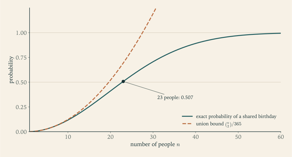
Figure 1.1 shows both the reason for the surprise and the limits of the union bound. For small groups the bound and the exact curve nearly coincide, because two different pairs rarely match at once; the probability grows like the number of pairs, roughly \(n^2/730\) . Once that quantity is no longer small, overlaps matter and only the exact complement calculation can be trusted.
The model deserves a remark. Real birthdays are not uniform over the year and the model ignores leap days. The conclusion is a statement about the model; whether it describes a real room is a separate, empirical question, and it happens that non-uniform birthdays make matches slightly more likely, not less.
1.5 Inclusion–exclusion when the complement does not help
The complement trick worked in the last two examples because “none” was a single, simple condition. When the events of interest overlap in a structured way and neither the union nor its complement can be counted directly, Theorem 1.4 does the work.
Example 1.5: Letters in the wrong envelopes
A secretary puts \(n\) letters into \(n\) addressed envelopes at random, all \(n!\) arrangements being equally likely. What is the probability that no letter is in its correct envelope?
Let \(A_i\) be the event that letter \(i\) is in its correct envelope. We want \(P\bigl((A_1\cup\dots\cup A_n)^c\bigr)\) . For any particular set of \(k\) letters, the arrangements that place all of them correctly are the \((n-k)!\) arrangements of the others, so each \(k\) -fold intersection has probability \((n-k)!/n!\) . There are \(\binom nk\) such intersections, and
Inclusion–exclusion gives
and therefore
For \(n=4\) this is \(1-1+\tfrac12-\tfrac16+\tfrac1{24}=\tfrac{3}{8}\) , which says that \(9\) of the \(24\) arrangements of four letters leave none in place; listing them confirms the count. The sum is a partial sum of the series for \(e^{-1}\) , and it converges very quickly: for \(n=7\) the probability is \(103/280\approx 0.36786\) , while \(1/e\approx 0.36788\) . So whether there are seven letters or seven thousand, the chance that none is correctly placed is about \(37\) percent. The answer barely depends on \(n\) , which few people would guess.
The union bound is useless here. Each \(A_i\) has probability \(1/n\) , so the bound on the probability of at least one correct letter is \(n\cdot(1/n)=1\) . The events overlap too much for the first term alone to say anything, and the alternating corrections are essential.
1.6 Sample spaces that are not finite
Nothing in Definition 1.2 requires \(\Omega\) to be finite, and two kinds of infinite sample space appear constantly.
Example 1.6: Waiting for the first head
Toss a fair coin until a head appears and record the number of tosses. The sample space is \(\Omega=\{1,2,3,\dots\}\) . The outcome \(k\) requires \(k-1\) tails followed by a head, one particular sequence among the \(2^k\) equally likely sequences of \(k\) tosses, so we assign \(P(\{k\})=2^{-k}\) . These numbers are positive and
so defining \(P(A)=\sum_{k\in A}2^{-k}\) for every \(A\subseteq\Omega\) gives a probability space: nonnegativity and normalization are clear, and countable additivity holds because a series of nonnegative terms may be summed in any grouping.
The outcomes are not equally likely, and no counting argument applies. Probabilities are sums of series. For instance, the probability that the first head arrives on an even-numbered toss is
The player who tosses first is therefore twice as likely to throw the first head as the player who tosses second.
What about the possibility that no head ever appears? It is not an outcome in \(\Omega\) , and to discuss it at all one needs a larger sample space whose outcomes are infinite sequences of tosses. That space has not been constructed here; building it, with a probability measure under which the tosses are independent and fair, is carried out in Measure-Theoretic Probability. Granting its existence, the event “no head in the first \(n\) tosses” has probability \(2^{-n}\) there, these events decrease as \(n\) grows, and by Theorem 1.5 their intersection, “no head ever”, has probability \(\lim 2^{-n}=0\) . That is the justification for leaving the outcome out: an event of probability zero can be added to or removed from a sample space without changing any calculation. Inside \(\Omega\) itself the corresponding events are the sets \(\{n+1,n+2,\dots\}\) , whose intersection is empty, and there Theorem 1.5 says only that \(P(\varnothing)=0\) , which is consistent and settles nothing about an endless run of tails.
A countably infinite sample space cannot carry equally likely outcomes. If every positive integer had the same probability \(c\) , countable additivity would force \(1=c+c+c+\cdots\) , which is impossible both for \(c=0\) and for \(c>0\) . There is no such thing as a uniformly random positive integer, and arguments that begin “choose an integer at random” need a different model.
The second kind of infinite sample space is a continuum. Spin a pointer and record the angle as a fraction of a full turn, a number in \(\Omega=[0,1)\) . Symmetry suggests that the probability of landing in an interval should be its length. Then every single point, being contained in intervals of arbitrarily small length, has probability zero, and yet the whole space has probability one. This is not a contradiction, because \([0,1)\) is not a countable union of points, and the axioms demand additivity only for countable families. It does mean that on a continuum probabilities cannot be built by adding up the probabilities of outcomes. They are built from intervals by integration, and that is the subject of Chapter 4.
The Chevalier’s question was about a single number. The next chapter asks how a probability should change when we learn that some event has occurred, which is the question on which all of statistics and most applications of probability depend.
Exercises
-
A fair coin is tossed three times. List the sample space of ordered results, and for the events \(A\) , “at least two heads”, and \(B\) , “the first toss is a head”, compute \(P(A)\) , \(P(B)\) , \(P(A\cap B)\) , and \(P(A\cup B)\) , checking the last against Theorem 1.3(f).
Answer
The sample space has the \(8\) equally likely sequences HHH, HHT, HTH, HTT, THH, THT, TTH, TTT. \(A=\{\text{HHH},\text{HHT},\text{HTH},\text{THH}\}\) and \(B\) is the set of four sequences beginning with H, so \(P(A)=P(B)=\tfrac12\) . \(A\cap B=\{\text{HHH},\text{HHT},\text{HTH}\}\) has probability \(\tfrac38\) , and \(A\cup B\) has five outcomes, probability \(\tfrac58=\tfrac12+\tfrac12-\tfrac38\) .
-
Using only the axioms and Theorem 1.3, prove that \(P(A\setminus B)=P(A)-P(A\cap B)\) for arbitrary events \(A\) and \(B\) , and deduce that the probability that exactly one of \(A\) and \(B\) occurs is \(P(A)+P(B)-2P(A\cap B)\) .
Solution
The set \(A\) is the disjoint union of \(A\cap B\) and \(A\setminus B\) : every outcome of \(A\) either lies in \(B\) or does not, and no outcome does both. Finite additivity, Theorem 1.3(b), gives \(P(A)=P(A\cap B)+P(A\setminus B)\) , which rearranges to
\[ P(A\setminus B)=P(A)-P(A\cap B). \]Exchanging the roles of the two events gives \(P(B\setminus A)=P(B)-P(A\cap B)\) . The event “exactly one of \(A\) and \(B\) occurs” is the union of \(A\setminus B\) and \(B\setminus A\) , and these are disjoint because an outcome in the first lies in \(A\) and an outcome in the second does not. Adding,
\[ P(\text{exactly one})=P(A)+P(B)-2P(A\cap B). \]As a check, adding \(P(A\cap B)\) to this recovers the formula for \(P(A\cup B)\) in Theorem 1.3(f), as it should, since “at least one” is the disjoint union of “exactly one” and “both”.
-
Prove that \(P(A\cap B)\ge P(A)+P(B)-1\) for all events \(A\) and \(B\) . If \(P(A)=0.9\) and \(P(B)=0.8\) , find the smallest and largest possible values of \(P(A\cap B)\) and describe a probability space attaining each.
Solution
By Theorem 1.3(f) and the fact that every probability is at most one,
\[ P(A\cap B)=P(A)+P(B)-P(A\cup B)\ge P(A)+P(B)-1 . \]With \(P(A)=0.9\) and \(P(B)=0.8\) this gives \(P(A\cap B)\ge 0.7\) . In the other direction \(A\cap B\subseteq B\) , so monotonicity gives \(P(A\cap B)\le 0.8\) . So the smallest possible value is \(0.7\) and the largest is \(0.8\) .
Both bounds are attained. Take \(\Omega=\{1,\dots,10\}\) with equally likely outcomes. For the upper bound let \(A=\{1,\dots,9\}\) and \(B=\{1,\dots,8\}\) , so that \(B\subseteq A\) and \(P(A\cap B)=P(B)=0.8\) . For the lower bound let \(A=\{1,\dots,9\}\) and \(B=\{3,\dots,10\}\) ; then \(A\cup B=\Omega\) and \(A\cap B=\{3,\dots,9\}\) has probability \(0.7\) . The lower bound is attained exactly when the union has probability one, that is, when the two complements, of probabilities \(0.1\) and \(0.2\) , do not overlap.
-
An integer is chosen from \(\{1,2,\dots,1000\}\) with all choices equally likely. Use inclusion–exclusion for three events to find the probability that it is divisible by at least one of \(2\) , \(3\) , and \(5\) .
Solution
Let \(A_2\) , \(A_3\) , \(A_5\) be the events that the chosen integer is divisible by \(2\) , \(3\) , \(5\) . The number of multiples of \(d\) in \(\{1,\dots,1000\}\) is the integer part of \(1000/d\) . An integer is divisible by two of these primes exactly when it is divisible by their product, so the intersections are counted by the multiples of \(6\) , \(10\) , \(15\) , and \(30\) :
\[ \lvert A_2\rvert=500,\quad \lvert A_3\rvert=333,\quad \lvert A_5\rvert=200,\quad \lvert A_2\cap A_3\rvert=166,\quad \lvert A_2\cap A_5\rvert=100,\quad \lvert A_3\cap A_5\rvert=66,\quad \lvert A_2\cap A_3\cap A_5\rvert=33 . \]Inclusion–exclusion gives
\[ \lvert A_2\cup A_3\cup A_5\rvert=500+333+200-166-100-66+33=734, \]so the probability is \(734/1000=0.734\) . The complement, \(0.266\) , is the probability that the integer has none of the three primes as a factor; it is close to \((1-\tfrac12)(1-\tfrac13)(1-\tfrac15)=\tfrac{4}{15}\approx 0.267\) , a coincidence that Chapter 2 explains through independence.
-
A fair die is rolled four times. Find the probability that the four results are all different, and the probability that some result appears at least twice.
Answer
All different: \(6\cdot5\cdot4\cdot3/6^4=360/1296=5/18\approx 0.278\) . Some result repeated: \(13/18\approx 0.722\) .
-
For a five-card poker hand find the probability of exactly one pair (two cards of one rank and three cards of three other distinct ranks) and the probability of a flush (five cards of one suit, straight flushes included), giving each as a fraction and a decimal.
Answer
One pair: \(13\binom42\binom{12}{3}4^3=1{,}098{,}240\) hands, probability \(352/833\approx 0.4226\) . Flush: \(4\binom{13}{5}=5148\) hands, probability \(33/16660\approx 0.00198\) . In the pair count the three unpaired ranks play the same role and are chosen as a set.
-
A student argues: “Two dice can show \(21\) different unordered combinations, and exactly one of them is a double six, so the probability of a double six is \(1/21\) .” Identify the false assumption, give the correct probability, and compute the correct probability that the two dice show different numbers.
Solution
The false assumption is that the \(21\) unordered combinations are equally likely. Proposition 1.6 applies only when a symmetry makes the outcomes being counted equally probable, and the symmetry of two fair dice acts on the \(36\) ordered pairs: each die independently has six equally likely faces. An unordered combination with two different numbers, such as \(\{2,5\}\) , corresponds to two ordered pairs and has probability \(2/36\) , while a double corresponds to one ordered pair and has probability \(1/36\) . As a check, \(15\cdot\tfrac{2}{36}+6\cdot\tfrac1{36}=1\) .
So the probability of a double six is \(1/36\) , not \(1/21\) . The probability that the dice show different numbers is \(1-6/36=5/6\) ; the student’s method would have given \(15/21=5/7\) .
-
In the birthday model of Example 1.4, find the smallest \(n\) for which a shared birthday has probability at least \(0.9\) . Then find the smallest number of other people needed for the probability that at least one of them shares your own birthday to reach one half, and explain in a sentence why the two answers differ so much.
Solution
Write \(q_n=\prod_{k=0}^{n-1}(365-k)/365\) for the probability that \(n\) birthdays are all different. Computing the product gives \(1-q_{40}\approx 0.8912\) and \(1-q_{41}\approx 0.9032\) , so the smallest \(n\) with a shared-birthday probability of at least \(0.9\) is \(n=41\) .
For the second question fix your own birthday. Each other person independently fails to share it with probability \(364/365\) , so among \(m\) others the probability that at least one shares it is \(1-(364/365)^m\) . This is at least one half when \(m\ge\ln 2/\ln(365/364)\approx 252.65\) , so \(m=253\) people are needed; indeed \(1-(364/365)^{253}\approx 0.5005\) while \(m=252\) gives \(0.4991\) .
The answers differ because the events differ. A match with one particular person involves only the \(m\) pairs that include that person, and the number of such pairs grows linearly. A match between any two people in a group of \(n\) involves \(\binom n2\) pairs, which grows quadratically; by a pleasant coincidence \(\binom{23}{2}=253\) .
-
A committee of four is chosen at random from seven women and five men. Find the probability that it has exactly two women, and the probability that it has at least one man.
Answer
Exactly two women: \(\binom72\binom52/\binom{12}{4}=210/495=14/33\) . At least one man: \(1-\binom74/\binom{12}{4}=1-35/495=92/99\) .
-
Five letters are placed at random in five addressed envelopes. Find the probability that exactly two letters are in their correct envelopes, using the count of arrangements of three letters with none correct.
Solution
All \(5!=120\) arrangements are equally likely. To have exactly two letters correct, choose which two are correct, \(\binom52=10\) ways, and then arrange the other three letters among their three envelopes so that none of them is correct. By Example 1.5 with \(n=3\) , the number of arrangements of three letters with none correct is \(3!\,(1-1+\tfrac12-\tfrac16)=2\) ; they are the two cyclic shifts. So there are \(10\cdot 2=20\) favourable arrangements and
\[ P(\text{exactly two correct})=\frac{20}{120}=\frac16 . \]The argument generalizes: the probability of exactly \(k\) correct among \(n\) is \(\frac{1}{k!}\) times the probability that \(n-k\) letters have none correct.
-
Complete the proof of Theorem 1.5 by writing out the decreasing case in full, and use it to show that if \(P(A_n)=1\) for every \(n\) then \(P\bigl(\bigcap_{n=1}^{\infty}A_n\bigr)=1\) .
Hint
For decreasing \(A_n\) , put \(C_n=A_n^c\) . Show the \(C_n\) increase, apply the increasing case to them, and use De Morgan’s law in the form \(\bigl(\bigcap A_n\bigr)^c=\bigcup A_n^c\) together with \(P(C_n)=1-P(A_n)\) . For the second part the sets \(A_n\) need not be decreasing, so apply the result to \(D_n=A_1\cap\dots\cap A_n\) , after proving \(P(D_n)=1\) from the union bound applied to complements.
-
Prove that there is no probability measure on the set of positive integers that gives every integer the same probability. Then give an example of a probability measure on the positive integers under which every integer has positive probability and odd integers together have probability \(2/3\) .
Solution
Suppose \(P\) is a probability measure on \(\{1,2,3,\dots\}\) with \(P(\{k\})=c\) for every \(k\) . The one-point events are pairwise disjoint and their union is the whole space, so countable additivity and normalization give
\[ 1=P(\Omega)=\sum_{k=1}^{\infty}c . \]If \(c=0\) the sum is \(0\) , and if \(c>0\) the partial sums \(nc\) are unbounded, so the series diverges. Neither equals \(1\) , so no such measure exists. Note that the argument uses countable additivity; finite additivity alone would not rule out \(c=0\) .
For the example take \(P(\{k\})=2^{-k}\) , the model of Example 1.6. Every integer has positive probability, the total is \(1\) , and the odd integers have total probability
\[ \sum_{m=0}^{\infty}2^{-(2m+1)}=\frac{1/2}{1-1/4}=\frac23 . \] -
A fair coin is tossed until the first head appears. Find the probability that the number of tosses is divisible by three.
Answer
\(\sum_{m\ge 1}2^{-3m}=\dfrac{1/8}{1-1/8}=\dfrac17\) .
-
Events \(A\) and \(B\) satisfy \(P(A)=0.5\) , \(P(B)=0.4\) , and \(P(A\cup B)=0.7\) . Draw a Venn diagram or a two-way table and find the probabilities that both occur, that \(A\) occurs alone, that exactly one occurs, and that neither occurs.
Answer
\(P(A\cap B)=0.5+0.4-0.7=0.2\) ; \(A\) alone, \(0.3\) ; \(B\) alone, \(0.2\) ; exactly one, \(0.5\) ; neither, \(1-0.7=0.3\) . The four regions of the diagram have probabilities \(0.3\) , \(0.2\) , \(0.2\) , \(0.3\) , which sum to one.
-
A system has \(20\) components, and each fails during a mission with probability at most \(0.001\) ; nothing is known about how failures are related. Give an upper bound for the probability that at least one component fails, and describe a probability space in which the bound is attained.
Hint
The union bound needs no information about dependence: the probability is at most \(20\times 0.001=0.02\) . For attainment you need the failure events to be pairwise disjoint, each with probability exactly \(0.001\) ; build a sample space with \(21\) outcomes, “component \(i\) alone fails” for each \(i\) and “nothing fails”.
-
The ten letter tiles of the word STATISTICS are arranged in a random order. Find the number of distinguishable arrangements and the probability that the arrangement begins and ends with the letter S.
Answer
The word has S three times, T three times, I twice, and A and C once each, so there are \(10!/(3!\,3!\,2!)=50{,}400\) distinguishable arrangements. Treating the ten tiles as distinct, the first position holds an S with probability \(3/10\) and then the last holds an S with probability \(2/9\) , so the probability is \(1/15\) . As a check, fixing S at both ends leaves \(8!/(3!\,2!)=3360\) distinguishable arrangements, and \(3360/50{,}400=1/15\) .
-
Derive the inclusion–exclusion formula for three events directly from Theorem 1.3(f), by writing \(A\cup B\cup C\) as \((A\cup B)\cup C\) and using the distributive law for sets.
Hint
Apply Theorem 1.3(f) to the two events \(A\cup B\) and \(C\) . The intersection term is \(P\bigl((A\cup B)\cap C\bigr)=P\bigl((A\cap C)\cup(B\cap C)\bigr)\) ; apply (f) again to it, noting that \((A\cap C)\cap(B\cap C)=A\cap B\cap C\) , and once more to \(P(A\cup B)\) .
-
A lottery draws six numbers without replacement from \(\{1,\dots,49\}\) , and a ticket lists six numbers. Find the probability that the ticket matches exactly three of the numbers drawn, and the probability that it matches none.
Answer
Exactly three: \(\binom63\binom{43}{3}/\binom{49}{6}=246{,}820/13{,}983{,}816\approx 0.01765\) . None: \(\binom{43}{6}/\binom{49}{6}\approx 0.4360\) .
-
Three balls are thrown independently into three labelled boxes, each ball equally likely to land in each box. Find the probabilities that no box is empty, that exactly one box is empty, and that two boxes are empty, and explain why the three occupancy patterns \((3,0,0)\) , \((2,1,0)\) , and \((1,1,1)\) are not equally likely.
Solution
The equally likely outcomes are the \(3^3=27\) assignments of a box to each of the three labelled balls. No box is empty exactly when the three balls go to three different boxes, which happens in \(3!=6\) assignments. Two boxes are empty exactly when all three balls share a box, \(3\) assignments. Everything else has exactly one empty box: \(27-6-3=18\) assignments. Directly, choose the empty box in \(3\) ways and assign the balls to the other two boxes in any of the \(2^3\) ways except the \(2\) that use only one box, giving \(3\cdot 6=18\) . Hence
\[ P(\text{no box empty})=\frac{6}{27}=\frac29,\qquad P(\text{one empty})=\frac{18}{27}=\frac23,\qquad P(\text{two empty})=\frac{3}{27}=\frac19 . \]The occupancy pattern \((1,1,1)\) arises from \(6\) assignments, a given pattern such as \((2,1,0)\) from \(3\) (choose which ball is alone), and \((3,0,0)\) from \(1\) . The symmetry of the experiment acts on the labelled balls, so the assignments are equally likely and the patterns are not. This is the unordered-with-replacement row of the table in Section 1.4.
-
Prove the countable union bound: for any sequence of events, \(P\bigl(\bigcup_{i=1}^{\infty}A_i\bigr)\le\sum_{i=1}^{\infty}P(A_i)\) . Deduce that a countable union of events of probability zero has probability zero.
Hint
Let \(U_n=A_1\cup\dots\cup A_n\) . The \(U_n\) increase to the full union, so Theorem 1.5 gives \(P(\bigcup A_i)=\lim P(U_n)\) . Bound \(P(U_n)\) by the finite union bound and then by the full series, whose partial sums increase. For the deduction, every term of the series is zero.