The lifetime of a lamp, the position at which a spinning pointer stops, the error in a measurement: quantities like these can take any value in an interval, and for them the probability mass function of Chapter 3 is useless. The probability that a lamp fails at exactly \(1000\) hours, to infinitely many decimal places, is zero, and the same is true of every other exact instant. Yet the lamp certainly fails at some instant, and the probability that it fails between \(900\) and \(1100\) hours is a perfectly sensible positive number. Probability is spread over the line like mass along a wire: no single point carries any, and yet intervals do.
Two questions organize the chapter. The first is how to describe such a distribution and compute with it; the answer is the distribution function and its derivative, the density. The second is subtler. If a random variable \(X\) has density \(f\) , what is the density of \(X^2\) , or of \(e^X\) , or of \(1/X\) ? Substituting into \(f\) gives the wrong answer every time, and understanding why is the main skill the chapter teaches.
4.1 The distribution function
One description works for every random variable, discrete or not.
Definition 4.1 (distribution function). The distribution function (or cumulative distribution function) of a random variable \(X\) is
Theorem 4.2 (properties of distribution functions). Let \(F\) be the distribution function of \(X\) . Then:
(a) \(F\) is nondecreasing;
(b) \(F(x)\to 0\) as \(x\to-\infty\) and \(F(x)\to 1\) as \(x\to+\infty\) ;
(c) \(F\) is right-continuous: \(F(x_n)\to F(x)\) whenever \(x_n\) decreases to \(x\) ;
(d) \(P(a<X\le b)=F(b)-F(a)\) for \(a<b\) ;
(e) \(P(X=x)=F(x)-F(x^-)\) , where \(F(x^-)\) is the limit of \(F\) from the left at \(x\) .
Proof. (a) and (d): for \(a<b\) the event \(\{X\le b\}\) is the disjoint union of \(\{X\le a\}\) and \(\{a<X\le b\}\) . (b) The events \(\{X\le n\}\) increase with \(n\) and their union is \(\Omega\) , so \(F(n)\to 1\) by continuity of probability, Theorem 1.5; since \(F\) is nondecreasing, \(F(x)\to 1\) . The events \(\{X\le -n\}\) decrease and their intersection is empty, so \(F(-n)\to 0\) . (c) If \(x_n\) decreases to \(x\) , the events \(\{X\le x_n\}\) decrease and their intersection is \(\{X\le x\}\) ; apply Theorem 1.5 again. (e) The events \(\{X\le x-1/n\}\) increase and their union is \(\{X<x\}\) , so \(P(X<x)=F(x^-)\) , and \(P(X=x)=P(X\le x)-P(X<x)\) .
Part (e) says that the jumps of \(F\) are exactly the point masses of \(X\) . A discrete random variable has a staircase for its distribution function, flat between its values and jumping by \(p_X(x)\) at each value \(x\) . At the other extreme, if \(F\) is continuous then every single value has probability zero. And nothing prevents a mixture of the two behaviours.
Example 4.1: Waiting at a traffic light
You arrive at a traffic light at a random moment. With probability \(0.4\) it is green and you do not wait. Otherwise it is red, and the remaining red time is equally likely to be anything between \(0\) and \(60\) seconds. Let \(W\) be your waiting time in seconds.
For \(0\le x\le 60\) , total probability gives
with \(F_W(x)=0\) for \(x<0\) and \(F_W(x)=1\) for \(x\ge 60\) . The function jumps from \(0\) to \(0.4\) at \(x=0\) and then rises continuously. By Theorem 4.2(e), \(P(W=0)=0.4\) , while every positive value has probability zero. The probability of waiting more than half a minute is \(1-F_W(30)=0.3\) .
This random variable is neither discrete nor does it have a density, and the distribution function handles it without complaint. Its mean is found by treating the two parts separately, as the law of total expectation of Chapter 6 will justify: the wait is \(0\) with probability \(0.4\) and otherwise averages \(30\) seconds, so the mean wait is \(0.6\cdot 30=18\) seconds.
4.2 Densities
Definition 4.3 (probability density function). A random variable \(X\) is continuous, with density \(f\) , if \(f\) is a nonnegative integrable function on \(\mathbb R\) such that
Four consequences follow at once. First, letting \(x\to\infty\) , a density has total integral one. Second, \(F_X\) is continuous, so \(P(X=x)=0\) for every \(x\) , and the four intervals with endpoints \(a<b\) all have the same probability:
Third, at every point where \(f\)
is continuous, the fundamental theorem of calculus gives \(F_X'(x)=f(x)\)
(math.calculus.fundamental-theorem-bridge): the density is the derivative of the distribution function. Fourth, changing \(f\)
at finitely many points changes no integral, so a density is determined only up to such changes, and it is pointless to ask whether a density is defined with \(<\)
or \(\le\)
at the ends of its support.
What does the number \(f(x)\) mean? For a small length \(h\) ,
So \(f(x)\) is probability per unit length near \(x\) . It is a rate, not a probability. It carries units, the reciprocal of the units of \(X\) , and it may exceed one: a random variable uniformly distributed on an interval of length \(\tfrac12\) has density equal to \(2\) throughout that interval.
The median of a continuous random variable is a number \(m\) with \(F_X(m)=\tfrac12\) , and more generally the quantile of order \(u\in(0,1)\) is a number \(x_u\) with \(F_X(x_u)=u\) . When \(F_X\) is strictly increasing on the set where it lies between \(0\) and \(1\) , each quantile is unique.
Example 4.2: A density on a bounded interval
Let \(X\) have density \(f(x)=c\,x(2-x)\) for \(0\le x\le 2\) and \(f(x)=0\) otherwise. Since \(\int_0^2 x(2-x)\,dx=4-\tfrac83=\tfrac43\) , normalization forces \(c=\tfrac34\) . The distribution function on \([0,2]\) is
which rises from \(F(0)=0\) to \(F(2)=1\) . Then
and by the symmetry of the density about \(x=1\) the same number is \(P(X>\tfrac32)\) , so \(P(\tfrac12<X\le\tfrac32)=1-\tfrac{10}{32}=\tfrac{11}{16}\) . The density at the centre is \(f(1)=\tfrac34\) . That is not the probability that \(X=1\) , which is zero; it says that an interval of small length \(h\) around \(1\) has probability about \(\tfrac34h\) .
Common mistake. Reading a density value as a probability. Statements such as “the probability that \(X\) equals \(1\) is \(f(1)\) ” are wrong in two ways: the probability is zero, and \(f(1)\) is not even constrained to be at most one. A density becomes a probability only when it is integrated over a set. When comparing two values, \(f(a)>f(b)\) does mean something: short intervals of equal length near \(a\) are more probable than near \(b\) .
4.3 Expectation, again
For a continuous random variable, sums become integrals.
Definition 4.4 (expectation of a continuous random variable). Let \(X\) have density \(f\) . If \(\int_{-\infty}^{\infty}\lvert x\rvert f(x)\,dx<\infty\) , then
If \(X\ge 0\) and the integral diverges, \(E[X]=\infty\) ; otherwise a divergent case is undefined.
Theorem 4.5 (expectation of a function; linearity). Let \(X\) have density \(f\) and let \(g\) be a function with \(\int\lvert g(x)\rvert f(x)\,dx<\infty\) . Then
Expectation is linear and monotone for all random variables with finite expectation, exactly as in Theorem 3.5.
The first statement is the continuous counterpart of Theorem 3.4, and it applies whether or not \(g(X)\) itself has a density. The second is the counterpart of Theorem 3.5. A proof of both in full generality defines expectation once for all random variables as an integral over the sample space, which is the business of Measure-Theoretic Probability; for a strictly monotone \(g\) the first statement follows from the change-of-variables theorem of Section 4.5, as Exercise 4.10 illustrates, and for two random variables with a joint density linearity will be immediate in Chapter 5. From here on we use both freely. Because variance was defined through expectation, Definition 3.8 carries over unchanged, and so do the two identities of Proposition 3.9, whose proofs used only linearity. The last clause of that proposition was proved by inspecting a sum over the mass function, and it needs a different argument here. Suppose \(\operatorname{Var}(X)=0\) . For each positive integer \(k\) the inequality \(\tfrac{1}{k^2}\mathbf 1_{\{\lvert X-\mu\rvert\ge 1/k\}}\le(X-\mu)^2\) holds at every outcome, and taking expectations gives \(P(\lvert X-\mu\rvert\ge\tfrac1k)\le k^2\operatorname{Var}(X)=0\) . The events \(\{\lvert X-\mu\rvert\ge\tfrac1k\}\) increase with \(k\) and their union is \(\{X\ne\mu\}\) , so \(P(X\ne\mu)=0\) by Theorem 1.5. The argument uses only monotonicity of expectation and so applies to every random variable. For a variable with a density it has a sharper consequence: since \(P(X=\mu)=0\) , the variance is never zero.
In Example 4.2 the mean is \(1\) by symmetry, and
The tail-sum formula of Chapter 3 also has a continuous form.
Proposition 4.6 (tail-integral formula). If \(X\ge 0\) has density \(f\) , then
Proof. Write \(P(X>t)=\int_t^{\infty}f(x)\,dx\) and exchange the order of integration over the region \(0\le t<x\) :
The exchange is legitimate because the integrand is nonnegative, by Tonelli’s theorem (math.measure-theory.tonelli-fubini-theorem).
Example 4.3: A symmetric density with no mean
The Cauchy density is
It integrates to one, since an antiderivative is \(\tfrac1\pi\arctan x\) , which runs from \(-\tfrac12\) to \(\tfrac12\) . It is symmetric about \(0\) , and it is tempting to declare its mean to be \(0\) . But
so the expectation is undefined. This is not a technicality. The value of \(\int_{-a}^{b}x f(x)\,dx\) depends on how \(a\) and \(b\) go to infinity: with \(b=a\) it tends to \(0\) , with \(b=2a\) it tends to \(\tfrac{1}{\pi}\ln 2\) . And the practical meaning of a mean also fails: Chapter 7 shows that averages of independent Cauchy observations do not settle down at all. The median, on the other hand, is \(0\) without any difficulty. Symmetry locates the median; it locates the mean only when there is one.
4.4 Uniform, exponential, and normal distributions
Three families account for most of the continuous models in this book.
The uniform distribution. \(X\sim\mathrm{Unif}(a,b)\) has density \(1/(b-a)\) on the interval \((a,b)\) and \(0\) elsewhere. Its distribution function rises linearly from \(0\) at \(a\) to \(1\) at \(b\) , the probability of a subinterval is proportional to its length, and
The variance comes from the case \(\mathrm{Unif}(0,1)\) , where \(E[X^2]=\tfrac13\) and so the variance is \(\tfrac13-\tfrac14=\tfrac1{12}\) , together with the scaling rule \(\operatorname{Var}(a+(b-a)U)=(b-a)^2\operatorname{Var}(U)\) .
The exponential distribution. \(T\sim\mathrm{Exp}(\lambda)\) , with rate \(\lambda>0\) , has density \(\lambda e^{-\lambda t}\) for \(t\ge 0\) . Its tail is the cleanest description:
By Proposition 4.6, \(E[T]=\int_0^{\infty}e^{-\lambda t}\,dt=1/\lambda\) . Two integrations by parts give \(E[T^2]=2/\lambda^2\) , so \(\operatorname{Var}(T)=1/\lambda^2\) : the standard deviation equals the mean. The exponential distribution is the continuous analogue of the geometric distribution, and it inherits the defining property.
Theorem 4.7 (lack of memory). If \(T\sim\mathrm{Exp}(\lambda)\) , then for all \(s,t\ge 0\) ,
Conversely, let \(T\) be a nonnegative continuous random variable with \(0<P(T>1)<1\) whose tail \(G(t)=P(T>t)\) satisfies \(G(s+t)=G(s)\,G(t)\) for all \(s,t\ge 0\) . Then \(T\) is exponential. The product form states lack of memory without a conditional probability, and so without presupposing that \(P(T>s)>0\) .
Proof. The conditional probability is \(e^{-\lambda(s+t)}/e^{-\lambda s}=e^{-\lambda t}\) . For the converse, the hypothesis gives \(G(1)=G(1/n)^n\) and \(G(m/n)=G(1/n)^m\) , so \(G(r)=G(1)^r\) for every positive rational \(r\) . Since \(G\) is nonincreasing and the rationals are dense, \(G(t)=G(1)^t\) for all \(t\ge 0\) , which is \(e^{-\lambda t}\) with \(\lambda=-\ln G(1)>0\) .
Example 4.4: A component that does not age
A lamp’s lifetime \(T\) , in hours, is exponential with mean \(1000\) , so \(\lambda=1/1000\) . The probability that it lasts beyond its mean lifetime is \(P(T>1000)=e^{-1}\approx 0.368\) , well under one half: the distribution is skewed, with a long right tail. The median solves \(e^{-m/1000}=\tfrac12\) , giving \(m=1000\ln 2\approx 693\) hours.
Now suppose the lamp has already burned for \(500\) hours. By Theorem 4.7,
A used lamp is as good as a new one. This is the right model for failures caused by external shocks that arrive at a constant rate, and the wrong model for anything that wears out: a real lamp that has survived \(500\) hours has usually used up some of its life. Whether lack of memory is plausible is the first thing to ask before adopting an exponential model.
The normal distribution. The density \(e^{-x^2/2}\) , suitably normalized, turns out to govern sums of many small independent effects; that is the central limit theorem of Chapter 8. Its normalizing constant requires a famous trick.
Lemma 4.8 (Gaussian integral).
Proof. Call the integral \(I\)
. It is finite and positive, since \(e^{-x^2/2}\le e^{-\lvert x\rvert+1/2}\)
. Write \(I^2\)
as a double integral over the plane and pass to polar coordinates, in which the area element \(dx\,dy\)
becomes \(r\,dr\,d\theta\)
(math.multivariable-calculus.change-of-variables-r2):
Definition 4.9 (normal distribution). The standard normal density and distribution function are
For real \(\mu\) and \(\sigma>0\) , a random variable \(X\) is normal with parameters \(\mu\) and \(\sigma^2\) , written \(X\sim N(\mu,\sigma^2)\) , if it has density
Proposition 4.10 (standardization). If \(Z\sim N(0,1)\) , then \(E[Z]=0\) and \(\operatorname{Var}(Z)=1\) . If \(X\sim N(\mu,\sigma^2)\) , then \((X-\mu)/\sigma\sim N(0,1)\) ; consequently \(E[X]=\mu\) , \(\operatorname{Var}(X)=\sigma^2\) , and
Proof. The function \(z\varphi(z)\) is odd and absolutely integrable, so \(E[Z]=0\) . Integrating by parts with \(u=z\) and \(dv=z\varphi(z)\,dz\) , so that \(v=-\varphi(z)\) ,
For the second statement, substitute \(u=(t-\mu)/\sigma\) in the integral of the density of \(X\) :
Then \(X=\mu+\sigma Z\) with \(Z\) standard normal, and the mean and variance follow from linearity and Proposition 3.9.
The function \(\Phi\) has no elementary formula and is tabulated or computed numerically. Symmetry of \(\varphi\) gives \(\Phi(-z)=1-\Phi(z)\) . A few values are worth knowing by heart.
| \(z\) | \(1\) | \(1.645\) | \(1.96\) | \(2\) | \(3\) |
|---|---|---|---|---|---|
| \(\Phi(z)\) | \(0.8413\) | \(0.9500\) | \(0.9750\) | \(0.9772\) | \(0.9987\) |
From them, the probability that a normal random variable falls within one, two, and three standard deviations of its mean is \(0.6827\) , \(0.9545\) , and \(0.9973\) .
Example 4.5: Reading normal probabilities
Scores on a test are modelled as \(X\sim N(100,15^2)\) . Every question about \(X\) is converted to a question about \(Z=(X-100)/15\) .
The probability of a score above \(130\) is \(P(Z>2)=1-\Phi(2)\approx 0.0228\) . The probability of a score between \(85\) and \(115\) is \(P(-1<Z<1)=2\Phi(1)-1\approx 0.6827\) . For the score that only one person in ten exceeds, we need \(z\) with \(\Phi(z)=0.9\) , which is \(z\approx 1.2816\) , so the score is \(100+15\cdot 1.2816\approx 119.2\) .
The pattern is always the same: subtract the mean, divide by the standard deviation, and consult \(\Phi\) . Standardizing is itself a transformation of a random variable, the simplest instance of the next section’s subject.
4.5 Transformations of a random variable
Given the distribution of \(X\) , what is the distribution of \(Y=g(X)\) ? There is one method that always works: compute the distribution function of \(Y\) directly, by rewriting the event \(\{g(X)\le y\}\) as an event about \(X\) , and differentiate if a density is wanted.
Example 4.6: The logarithm of a uniform variable
Let \(U\sim\mathrm{Unif}(0,1)\) and \(Y=-\ln U\) . Since \(0<U<1\) , the values of \(Y\) are positive. For \(y>0\) ,
because \(U\) is uniform and \(e^{-y}\) lies in \((0,1)\) . Differentiating, \(f_Y(y)=e^{-y}\) for \(y>0\) : the variable \(Y\) is exponential with rate \(1\) . Notice where care was needed: the function \(-\ln\) is decreasing, so the inequality reversed when it was undone. A uniform density, flat on \((0,1)\) , has become a density that is far from flat on \((0,\infty)\) . The values of \(U\) near \(0\) , a short interval, are spread by the logarithm over the whole far tail.
The example is a special case of a general principle that is the basis of computer simulation.
Theorem 4.11 (inverse distribution function). Let \(F\) be a distribution function that is continuous and strictly increasing on an interval \((\alpha,\beta)\) , with \(F(x)\to 0\) as \(x\to\alpha\) and \(F(x)\to 1\) as \(x\to\beta\) , so that \(F\) has an inverse \(F^{-1}:(0,1)\to(\alpha,\beta)\) .
(a) If \(U\sim\mathrm{Unif}(0,1)\) , then \(X=F^{-1}(U)\) has distribution function \(F\) .
(b) If \(X\) has distribution function \(F\) , then \(F(X)\sim\mathrm{Unif}(0,1)\) .
Proof. (a) For \(x\in(\alpha,\beta)\) , applying the increasing function \(F\) to both sides, \(P(F^{-1}(U)\le x)=P(U\le F(x))=F(x)\) . (b) For \(u\in(0,1)\) , \(P(F(X)\le u)=P(X\le F^{-1}(u))=F(F^{-1}(u))=u\) .
So a single source of uniform random numbers suffices to simulate any such distribution: to produce an exponential variable with rate \(\lambda\) , solve \(1-e^{-\lambda x}=u\) to get \(x=-\ln(1-u)/\lambda\) , and feed in uniform \(u\) .
When \(g\) is monotone and smooth, the differentiation can be done once and for all.
Theorem 4.12 (change of variables, monotone case). Let \(X\) have a density \(f_X\) that vanishes outside an open interval \(I\) . Let \(g\) be strictly monotone on \(I\) with a continuous derivative that is never zero, let \(J=g(I)\) , and let \(h:J\to I\) be the inverse of \(g\) . Then \(Y=g(X)\) has density
Proof. The inverse \(h\) is strictly monotone and continuously differentiable, with \(h'(y)=1/g'(h(y))\) . Suppose first that \(g\) is increasing, and let \(I=(a,b)\) and \(J=(c,d)\) . For \(y\in J\) , substituting \(x=h(u)\) ,
If \(g\) is decreasing, then \(h\) is decreasing, \(\{g(X)\le y\}=\{X\ge h(y)\}\) , and the same substitution, in which \(u\) runs from \(y\) down to \(c\) as \(x\) runs from \(h(y)\) up to \(b\) , gives
In both cases \(F_Y(y)\) is the integral from \(c\) to \(y\) of \(f_X(h(u))\lvert h'(u)\rvert\) . Since \(Y\) takes values in \(J\) , this function is a density for \(Y\) .
The factor \(\lvert h'(y)\rvert\) is what the naive substitution \(f_X(h(y))\) leaves out, and the reason for it is conservation of probability. A short interval of length \(dx\) at \(x\) is mapped by \(g\) to an interval of length \(dy=\lvert g'(x)\rvert\,dx\) at \(y\) . Both carry the same probability, so
Where \(g\) stretches the line, probability is diluted and the density falls; where \(g\) compresses it, the density rises. Densities transform like rates, not like functions.
Example 4.7: The lognormal density
Let \(Z\sim N(0,1)\) and \(Y=e^{Z}\) . Here \(g(z)=e^z\) is increasing on \(\mathbb R\) with \(J=(0,\infty)\) , and \(h(y)=\ln y\) , \(h'(y)=1/y\) . By Theorem 4.12,
This is the lognormal density. Because \(g\) is increasing, quantiles map to quantiles: the median of \(Y\) is \(e^0=1\) . Probabilities of corresponding intervals agree,
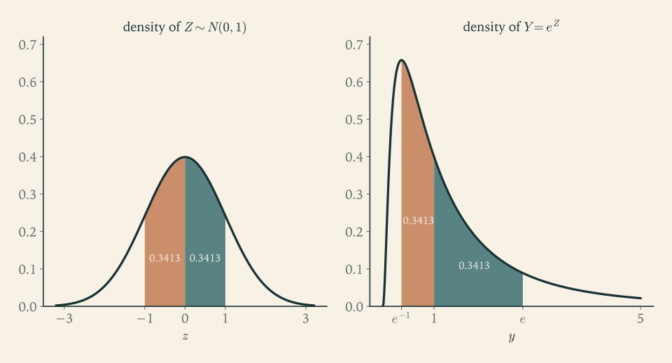
Figure 4.1 shows the two bands before and after. The intervals \((-1,0)\) and \((0,1)\) have equal length and equal probability under the symmetric normal density. Their images \((e^{-1},1)\) and \((1,e)\) have lengths about \(0.63\) and \(1.72\) . Equal areas over unequal bases force unequal heights, which is the factor \(1/y\) . The symmetric bell has become a skewed density whose peak, at \(y=e^{-1}\) , lies to the left of its median.
When \(g\) is not monotone, several values of \(x\) may be sent to the same \(y\) , and each contributes.
Theorem 4.13 (change of variables with several branches). Let \(X\) have a density \(f_X\) that vanishes outside a set which, apart from finitely many points, is a union of disjoint open intervals \(I_1,\dots,I_m\) . Suppose that on each \(I_j\) the function \(g\) is strictly monotone with a continuous nonvanishing derivative, and let \(h_j\) be the inverse of \(g\) on \(I_j\) . Then \(Y=g(X)\) has density
Proof. The finitely many exceptional points have probability zero, so \(F_Y(y)=\sum_j P(X\in I_j,\ g(X)\le y)\) . The argument of Theorem 4.12, applied on each \(I_j\) separately, writes the \(j\) -th term as the integral up to \(y\) of \(f_X(h_j(u))\lvert h_j'(u)\rvert\) over those \(u\) that lie in \(g(I_j)\) . Adding the \(m\) integrals gives the integral of the stated sum.
Example 4.8: The square of a uniform variable on an asymmetric interval
Let \(X\sim\mathrm{Unif}(-1,2)\) , with density \(\tfrac13\) on \((-1,2)\) , and \(Y=X^2\) . The function \(g(x)=x^2\) is decreasing on \(I_1=(-1,0)\) and increasing on \(I_2=(0,2)\) , with \(g(I_1)=(0,1)\) and \(g(I_2)=(0,4)\) . The inverses are \(h_1(y)=-\sqrt y\) and \(h_2(y)=\sqrt y\) , each with \(\lvert h_j'(y)\rvert=\dfrac{1}{2\sqrt y}\) .
For \(0<y<1\) both branches contribute, and for \(1<y<4\) only the second does:
and \(f_Y(y)=0\) otherwise. As a check,
The distribution-function method gives the same result and is a good way to verify the branch structure: for \(0<y<1\) , \(P(X^2\le y)=P(-\sqrt y\le X\le\sqrt y)=\tfrac{2\sqrt y}{3}\) , while for \(1\le y<4\) the lower limit \(-\sqrt y\) falls outside the support and \(P(X^2\le y)=P(-1<X\le\sqrt y)=\tfrac{\sqrt y+1}{3}\) . Differentiating each piece recovers the two formulas. The density jumps down at \(y=1\) , where the left branch runs out, and it is unbounded near \(y=0\) , where \(g\) is flat and compresses a neighbourhood of \(x=0\) into a much shorter interval. An unbounded density is harmless as long as it is integrable.
Common mistake. Writing \(f_Y(y)=f_X(h(y))\) , without the derivative factor, or using only one branch. For \(X\sim\mathrm{Unif}(0,1)\) and \(Y=X^2\) the first error gives the “density” \(1\) on \((0,1)\) , which would make \(Y\) uniform; but \(P(Y\le\tfrac14)=P(X\le\tfrac12)=\tfrac12\) , not \(\tfrac14\) . Two checks catch nearly every error of this kind. Integrate the proposed density: it must give one. And compute one probability, such as \(P(Y\le y_0)\) for a convenient \(y_0\) , directly from the distribution of \(X\) .
4.6 Moment generating functions
The probability generating function of Chapter 3 is available only for nonnegative integer values. Replacing \(s^X\) by \(e^{tX}\) gives a transform that makes sense for any random variable.
Definition 4.14 (moment generating function). The moment generating function of a random variable \(X\) is
defined for those real \(t\) at which the expectation is finite. We say that the moment generating function of \(X\) exists if \(M_X(t)\) is finite for all \(t\) in some open interval containing \(0\) .
Always \(M_X(0)=1\) . The expectation is a sum \(\sum_x e^{tx}p_X(x)\) for a discrete variable and an integral \(\int e^{tx}f_X(x)\,dx\) for a continuous one. For a nonnegative integer-valued variable, \(M_X(t)=G_X(e^t)\) , so the two transforms carry the same information.
Theorem 4.15 (moments from the generating function). Suppose \(M_X(t)\) is finite for \(\lvert t\rvert<\delta\) , where \(\delta>0\) . Then \(E[\lvert X\rvert^k]<\infty\) for every \(k\ge 1\) , and
Proof. Fix \(t\)
with \(0<\lvert t\rvert<\delta\)
. Since \(e^{\lvert tx\rvert}\le e^{tx}+e^{-tx}\)
, we have \(E[e^{\lvert tX\rvert}]\le M_X(t)+M_X(-t)<\infty\)
. Each term of the exponential series is at most the whole sum, \(\lvert tx\rvert^k/k!\le e^{\lvert tx\rvert}\)
, so \(E[\lvert X\rvert^k]\le k!\,E[e^{\lvert tX\rvert}]/\lvert t\rvert^k<\infty\)
. The partial sums of \(\sum_k(tX)^k/k!\)
converge to \(e^{tX}\)
and are bounded in absolute value by \(e^{\lvert tX\rvert}\)
, which has finite expectation; the dominated convergence theorem (math.measure-theory.dominated-convergence-theorem) therefore allows the expectation to be taken term by term, which is the series formula. A power series with positive radius of convergence may be differentiated term by term, and its \(k\)
-th derivative at \(0\)
is \(k!\)
times its \(k\)
-th coefficient.
The \(k\) -th moment is the \(k\) -th derivative at zero, or equivalently \(k!\) times the coefficient of \(t^k\) ; whichever is easier to extract.
Theorem 4.16 (uniqueness). If \(M_X(t)=M_Y(t)<\infty\) for all \(t\) in an open interval containing \(0\) , then \(X\) and \(Y\) have the same distribution.
The proof requires analytic tools beyond this course and is given in Measure-Theoretic Probability. We use the theorem as follows: if a computation produces a function recognizable as the moment generating function of a known distribution, that distribution has been identified. The hypothesis of an interval around \(0\) matters; agreement of all moments is not enough by itself.
Proposition 4.17 (affine changes). For real \(a\) and \(b\) , \(M_{aX+b}(t)=e^{bt}M_X(at)\) wherever the right-hand side is finite.
Proof. \(E[e^{t(aX+b)}]=e^{bt}E[e^{(at)X}]\) , by linearity.
Example 4.9: Three generating functions and what they yield
Exponential. For \(T\sim\mathrm{Exp}(\lambda)\) and \(t<\lambda\) ,
For \(t\ge\lambda\) the integral diverges; the function exists in the sense of Definition 4.14 because \((-\lambda,\lambda)\) is an interval around \(0\) . Comparing the coefficient \(1/\lambda^k\) with \(E[T^k]/k!\) gives every moment at once: \(E[T^k]=k!/\lambda^k\) . In particular \(E[T]=1/\lambda\) and \(E[T^2]=2/\lambda^2\) , as found in Section 4.4.
Standard normal. Completing the square in the exponent, \(tz-\tfrac12z^2=\tfrac12t^2-\tfrac12(z-t)^2\) , so
the remaining integrand being the \(N(t,1)\) density. Expanding, \(e^{t^2/2}=1+\tfrac{t^2}{2}+\tfrac{t^4}{8}+\tfrac{t^6}{48}+\cdots\) . The odd moments vanish, and the even ones are \(E[Z^2]=2!\cdot\tfrac12=1\) , \(E[Z^4]=4!\cdot\tfrac18=3\) , and \(E[Z^6]=6!\cdot\tfrac1{48}=15\) .
General normal. If \(X=\mu+\sigma Z\) , Proposition 4.17 gives
By Theorem 4.16 this function is a signature: any random variable whose moment generating function is the exponential of a quadratic \(\mu t+\tfrac12\sigma^2t^2\) is \(N(\mu,\sigma^2)\) . Evaluating at \(t=1\) with \(\mu=0\) and \(\sigma=1\) gives the mean of the lognormal variable of Example 4.7 without integrating its density: \(E[e^{Z}]=M_Z(1)=e^{1/2}\approx 1.649\) , noticeably larger than its median \(1\) .
Not every distribution has a moment generating function. The Cauchy distribution has none, since it has no mean. More subtly, the lognormal variable \(Y=e^Z\) has all its moments, \(E[Y^k]=M_Z(k)=e^{k^2/2}\) , and yet \(E[e^{tY}]=\infty\) for every \(t>0\) , because \(e^{te^{z}}\) grows faster than \(\varphi(z)\) decays. Existence of the moment generating function is a strong condition: it says the tails of the distribution decay at least exponentially fast.
Three applications lie ahead. In Chapter 5 the moment generating function of a sum of independent random variables is shown to be the product of theirs, which identifies the distributions of many sums. In Chapter 7 it produces exponentially small bounds on tail probabilities. And in Chapter 8 it carries the proof of the central limit theorem.
Exercises
-
A random variable \(X\) has distribution function \(F(x)=0\) for \(x<0\) , \(F(x)=x/4\) for \(0\le x<1\) , \(F(x)=\tfrac12\) for \(1\le x<2\) , and \(F(x)=1\) for \(x\ge 2\) . Find \(P(X=1)\) , \(P(X=2)\) , \(P(X<1)\) , and \(P(\tfrac12<X\le 1)\) , and compute \(E[X]\) by splitting \(X\) into its continuous and discrete parts.
Solution
By Theorem 4.2(e) the point masses are the jumps of \(F\) . At \(x=1\) the left limit is \(\tfrac14\) and the value is \(\tfrac12\) , so \(P(X=1)=\tfrac14\) . At \(x=2\) the left limit is \(\tfrac12\) and the value is \(1\) , so \(P(X=2)=\tfrac12\) . Next, \(P(X<1)=F(1^-)=\tfrac14\) , and by Theorem 4.2(d),
\[ P\bigl(\tfrac12<X\le 1\bigr)=F(1)-F\bigl(\tfrac12\bigr)=\tfrac12-\tfrac18=\tfrac38 . \]The remaining probability \(\tfrac14\) is spread over \((0,1)\) with density \(F'(x)=\tfrac14\) . For the mean, condition on which part \(X\) falls in, or equivalently add the contribution of the density to that of the atoms:
\[ E[X]=\int_0^1x\cdot\tfrac14\,dx+1\cdot\tfrac14+2\cdot\tfrac12=\tfrac18+\tfrac14+1=\tfrac{11}{8}. \]The three pieces of probability, \(\tfrac14+\tfrac14+\tfrac12\) , sum to one, which confirms that nothing has been missed.
-
Let \(X\) have density \(f(x)=c/x^3\) for \(x\ge 1\) and \(0\) otherwise. Find \(c\) , the distribution function, the median, and the mean, and show that the variance is infinite.
Solution
Normalization: \(\int_1^{\infty}c\,x^{-3}\,dx=c/2\) , so \(c=2\) . For \(x\ge 1\) ,
\[ F(x)=\int_1^x2t^{-3}\,dt=1-\frac{1}{x^2}, \]and \(F(x)=0\) for \(x<1\) . The median solves \(1-1/m^2=\tfrac12\) , so \(m=\sqrt2\approx 1.414\) . The mean is
\[ E[X]=\int_1^{\infty}x\cdot 2x^{-3}\,dx=\int_1^{\infty}2x^{-2}\,dx=2 . \]For the second moment, \(E[X^2]=\int_1^{\infty}2x^{-1}\,dx=\lim_{b\to\infty}2\ln b=\infty\) , so the variance is infinite. This is a Pareto distribution. Its tail \(P(X>x)=x^{-2}\) decays like a power, slowly enough that the mean exists and the variance does not; the mean, \(2\) , is well above the median because of that heavy tail.
-
Let \(X\) have density \(f(x)=c\,e^{-\lvert x\rvert}\) on the whole real line. Find \(c\) , \(P(\lvert X\rvert>1)\) , and \(\operatorname{Var}(X)\) .
Answer
\(c=\tfrac12\) . \(P(\lvert X\rvert>1)=\int_1^{\infty}e^{-x}\,dx=e^{-1}\approx 0.368\) . The mean is \(0\) by symmetry and \(E[X^2]=\int_0^{\infty}x^2e^{-x}\,dx=2\) , so the variance is \(2\) .
-
A bus arrives at a time uniformly distributed over the next ten minutes. Find the probability that you wait more than seven minutes given that you have already waited four, compare it with the unconditional probability of waiting more than three minutes, and say what this shows about the uniform distribution.
Answer
\(P(W>7\mid W>4)=\dfrac{0.3}{0.6}=\dfrac12\) , while \(P(W>3)=0.7\) . Having waited makes a further three-minute wait less likely: the uniform distribution has memory, because the bus must arrive by a fixed deadline.
-
A service time is exponential with mean five minutes. Find the probability that it exceeds ten minutes, the probability that it is under three minutes, the probability that it exceeds ten minutes given that it has exceeded four, and the time that it exceeds with probability \(0.1\) .
Answer
With \(\lambda=\tfrac15\) per minute: \(P(T>10)=e^{-2}\approx 0.1353\) ; \(P(T<3)=1-e^{-0.6}\approx 0.4512\) ; \(P(T>10\mid T>4)=P(T>6)=e^{-1.2}\approx 0.3012\) ; and \(e^{-t/5}=0.1\) gives \(t=5\ln 10\approx 11.51\) minutes.
-
Let \(T_n\) be geometric with success probability \(\lambda/n\) , where \(\lambda>0\) is fixed and \(n>\lambda\) . Show that \(P(T_n/n>t)\to e^{-\lambda t}\) for every \(t>0\) , and interpret the result as a statement about trials performed \(n\) times per unit of time.
Solution
The event \(\{T_n/n>t\}\) is \(\{T_n>nt\}\) , and since \(T_n\) is an integer this is \(\{T_n>m\}\) with \(m\) the integer part of \(nt\) . The geometric tail gives
\[ P(T_n/n>t)=\Bigl(1-\frac{\lambda}{n}\Bigr)^{m},\qquad nt-1<m\le nt . \]Because \(0<1-\lambda/n<1\) , this lies between \((1-\lambda/n)^{nt}\) and \((1-\lambda/n)^{nt-1}\) . Now \((1-\lambda/n)^{n}\to e^{-\lambda}\) , so \((1-\lambda/n)^{nt}\to e^{-\lambda t}\) , and the extra factor \((1-\lambda/n)^{-1}\) tends to \(1\) . Both bounds converge to \(e^{-\lambda t}\) , hence so does the probability.
Interpretation: perform \(n\) independent trials per unit of time, each succeeding with the small probability \(\lambda/n\) , so that the expected number of successes per unit time is \(\lambda\) . Measured in units of time, the wait for the first success is \(T_n/n\) , and as the trials become more frequent and individually less likely, its distribution approaches \(\mathrm{Exp}(\lambda)\) . The exponential distribution is the continuous-time limit of the geometric, just as the Poisson distribution of Theorem 3.12 is the limit of the binomial count in the same scheme.
-
Heights in a population are modelled as normal with mean \(170\) and standard deviation \(8\) , in centimetres. Find the probability that a height exceeds \(186\) , the probability that it lies between \(160\) and \(175\) , and the height exceeded by five percent of the population.
Solution
Standardize with \(Z=(X-170)/8\) . For the first probability, \(186\) is two standard deviations above the mean:
\[ P(X>186)=P(Z>2)=1-\Phi(2)\approx 0.0228 . \]For the second, \(160\) and \(175\) correspond to \(z=-1.25\) and \(z=0.625\) , so
\[ P(160<X<175)=\Phi(0.625)-\Phi(-1.25)\approx 0.7340-0.1056=0.6284 . \]For the height exceeded by five percent we need \(\Phi(z)=0.95\) , that is \(z\approx 1.645\) , giving \(170+1.645\cdot 8\approx 183.2\) centimetres. The interval in the second part is not symmetric about the mean, so the shortcut \(2\Phi(z)-1\) does not apply; each endpoint must be standardized separately, and the negative one handled with \(\Phi(-z)=1-\Phi(z)\) .
-
For \(Z\sim N(0,1)\) show that \(E[\lvert Z\rvert]=\sqrt{2/\pi}\) , and show that the density of \(N(\mu,\sigma^2)\) has its inflection points at \(\mu-\sigma\) and \(\mu+\sigma\) .
Hint
For the first part use symmetry to write \(E[\lvert Z\rvert]=2\int_0^{\infty}z\varphi(z)\,dz\) and note that \(z\varphi(z)\) is the derivative of \(-\varphi(z)\) . For the second, differentiate the standard normal density twice to get \(\varphi''(z)=(z^2-1)\varphi(z)\) , which changes sign at \(z=-1\) and \(z=1\) , and transfer the result through \(x=\mu+\sigma z\) .
-
Let \(X\sim\mathrm{Unif}(0,1)\) and \(Y=X^2\) . A student writes “the density of \(Y\) is \(f_X(\sqrt y)=1\) for \(0<y<1\) ”. Find the correct density by the distribution-function method, confirm it with Theorem 4.12, verify that it integrates to one, and exhibit a probability that the student’s density gets wrong.
Solution
For \(0<y<1\) , since \(X>0\) ,
\[ F_Y(y)=P(X^2\le y)=P(X\le\sqrt y)=\sqrt y, \]and differentiating gives \(f_Y(y)=\dfrac{1}{2\sqrt y}\) for \(0<y<1\) . Theorem 4.12 agrees: \(g(x)=x^2\) is increasing on \((0,1)\) with inverse \(h(y)=\sqrt y\) and \(h'(y)=\dfrac{1}{2\sqrt y}\) , so \(f_Y(y)=f_X(\sqrt y)\,h'(y)=\dfrac{1}{2\sqrt y}\) . It integrates to one: \(\int_0^1\dfrac{dy}{2\sqrt y}=\bigl[\sqrt y\bigr]_0^1=1\) .
The student omitted the factor \(h'(y)\) . The student’s density would make \(Y\) uniform and give \(P(Y\le\tfrac14)=\tfrac14\) . The true value is \(P(Y\le\tfrac14)=P(X\le\tfrac12)=\tfrac12\) . Squaring compresses the interval \((0,\tfrac12)\) into \((0,\tfrac14)\) , so half the probability sits on the first quarter of the range, and the density must be large near \(0\) to account for it.
-
Let \(X\sim\mathrm{Exp}(\lambda)\) and \(Y=\sqrt X\) . Find the density of \(Y\) , and compute \(E[Y]\) in two ways: from the density of \(Y\) , and as \(E[\sqrt X]\) from the density of \(X\) by Theorem 4.5.
Solution
The function \(g(x)=\sqrt x\) is increasing on \((0,\infty)\) with inverse \(h(y)=y^2\) and \(h'(y)=2y\) . By Theorem 4.12,
\[ f_Y(y)=f_X(y^2)\cdot 2y=2\lambda y\,e^{-\lambda y^2},\qquad y>0 . \]First computation of the mean, from this density: integrate by parts with \(u=y\) and \(dv=2\lambda ye^{-\lambda y^2}dy\) , so \(v=-e^{-\lambda y^2}\) :
\[ E[Y]=\int_0^{\infty}y\cdot 2\lambda y\,e^{-\lambda y^2}\,dy=\Bigl[-ye^{-\lambda y^2}\Bigr]_0^{\infty}+\int_0^{\infty}e^{-\lambda y^2}\,dy=\frac12\sqrt{\frac{\pi}{\lambda}} . \]The last integral is half of a Gaussian integral: substituting \(y=u/\sqrt{2\lambda}\) in Lemma 4.8 gives \(\int_{-\infty}^{\infty}e^{-\lambda y^2}dy=\sqrt{\pi/\lambda}\) .
Second computation, by Theorem 4.5: \(E[\sqrt X]=\int_0^{\infty}\sqrt x\,\lambda e^{-\lambda x}\,dx\) . The substitution \(x=y^2\) , \(dx=2y\,dy\) turns this into \(\int_0^{\infty}y\cdot 2\lambda ye^{-\lambda y^2}dy\) , the very integral just evaluated. That is exactly how Theorem 4.5 follows from Theorem 4.12 for a monotone \(g\) . For \(\lambda=1\) the mean is \(\sqrt\pi/2\approx 0.886\) .
-
Let \(X\) be uniformly distributed on \((-\tfrac{\pi}{2},\tfrac{\pi}{2})\) and \(Y=\tan X\) . Show that \(Y\) has the Cauchy density of Example 4.3, and describe a physical experiment with a spinning pointer and a straight wall that this models.
Answer
On \((-\tfrac\pi2,\tfrac\pi2)\) the tangent is increasing with inverse \(h(y)=\arctan y\) and \(h'(y)=\dfrac{1}{1+y^2}\) , and \(f_X=\dfrac1\pi\) , so \(f_Y(y)=\dfrac{1}{\pi(1+y^2)}\) . A pointer pivoted at distance one from a long straight wall and spun to a uniformly random angle points at a spot on the wall whose position has this distribution.
-
Let \(Z\sim N(0,1)\) and \(Y=Z^2\) . Use Theorem 4.13 to find the density of \(Y\) , and compute \(P(Y\le 1)\) from a value of \(\Phi\) .
Answer
Both branches \(h(y)=\pm\sqrt y\) have \(\lvert h'(y)\rvert=\dfrac{1}{2\sqrt y}\) , so \(f_Y(y)=2\varphi(\sqrt y)\dfrac{1}{2\sqrt y}=\dfrac{1}{\sqrt{2\pi y}}e^{-y/2}\) for \(y>0\) . \(P(Y\le 1)=P(-1\le Z\le 1)=2\Phi(1)-1\approx 0.6827\) .
-
Let \(U\sim\mathrm{Unif}(0,1)\) and \(Y=1/U\) . Find the density of \(Y\) and show that \(E[Y]=\infty\) .
Answer
\(h(y)=1/y\) on \(y>1\) , \(\lvert h'(y)\rvert=1/y^2\) , so \(f_Y(y)=1/y^2\) for \(y>1\) . Then \(E[Y]=\int_1^{\infty}y^{-1}\,dy=\infty\) ; equivalently \(E[1/U]=\int_0^1u^{-1}\,du=\infty\) .
-
Use Theorem 4.11 to express, as functions of a uniform variable \(U\) on \((0,1)\) , a random variable with density \(2x\) on \((0,1)\) and a random variable with the density of Exercise 2.
Answer
For density \(2x\) , \(F(x)=x^2\) on \((0,1)\) and \(X=\sqrt U\) . For the density of Exercise 2, \(F(x)=1-x^{-2}\) , so \(X=(1-U)^{-1/2}\) ; since \(1-U\) is also uniform, \(X=U^{-1/2}\) serves equally well.
-
A lamp with \(\mathrm{Exp}(\lambda)\) lifetime \(T\) is replaced when it fails or at age \(c\) , whichever comes first. Use Theorem 4.5 with \(g(t)=\min(t,c)\) to find the expected time \(E[\min(T,c)]\) until replacement, show that it equals \(\int_0^c P(T>t)\,dt\) , evaluate it for \(\lambda=1\) and \(c=2\) , and check the limits as \(c\to 0\) and \(c\to\infty\) .
Solution
By Theorem 4.5 with \(g(t)=\min(t,c)\) , which equals \(t\) for \(t\le c\) and \(c\) beyond,
\[ E[\min(T,c)]=\int_0^{c}t\,\lambda e^{-\lambda t}\,dt+c\int_c^{\infty}\lambda e^{-\lambda t}\,dt . \]Integrate the first term by parts with \(u=t\) and \(v=-e^{-\lambda t}\) : it equals \(-ce^{-\lambda c}+\int_0^ce^{-\lambda t}\,dt\) . The second term is \(ce^{-\lambda c}\) , which cancels the boundary term, leaving
\[ E[\min(T,c)]=\int_0^{c}e^{-\lambda t}\,dt=\int_0^cP(T>t)\,dt=\frac{1-e^{-\lambda c}}{\lambda}. \]This is the tail-integral formula for the variable \(\min(T,c)\) , whose tail equals that of \(T\) below \(c\) and vanishes above; the formula holds here although \(\min(T,c)\) has an atom at \(c\) and no density. For \(\lambda=1\) and \(c=2\) the value is \(1-e^{-2}\approx 0.8647\) . As \(c\to 0\) the expression behaves like \(c\) , since replacement at age \(c\) is then nearly certain, and as \(c\to\infty\) it tends to \(1/\lambda\) , the mean lifetime.
-
Find the moment generating function of \(U\sim\mathrm{Unif}(0,1)\) , expand it as a power series, and read off \(E[U^k]\) for every \(k\) .
Answer
\(M(t)=\int_0^1e^{tx}\,dx=\dfrac{e^t-1}{t}\) for \(t\ne 0\) , and \(M(0)=1\) . The series is \(\sum_{k\ge 0}\dfrac{t^k}{(k+1)!}\) , so \(E[U^k]/k!=1/(k+1)!\) and \(E[U^k]=\dfrac{1}{k+1}\) , as direct integration confirms.
-
A random variable \(X\) has moment generating function \(M(t)=e^{3t+2t^2}\) for all real \(t\) . Identify its distribution, and find \(E[X^2]\) and \(P(X>5)\) .
Solution
The exponent is \(\mu t+\tfrac12\sigma^2t^2\) with \(\mu=3\) and \(\tfrac12\sigma^2=2\) , so \(\sigma^2=4\) . The function is finite for all \(t\) , in particular on an interval around \(0\) , so by the uniqueness theorem, Theorem 4.16, \(X\sim N(3,4)\) , with standard deviation \(2\) .
Then \(E[X^2]=\operatorname{Var}(X)+E[X]^2=4+9=13\) . The same value comes from the derivatives: \(M'(t)=(3+4t)M(t)\) and \(M''(t)=\bigl(4+(3+4t)^2\bigr)M(t)\) , so \(M''(0)=4+9=13\) . Finally, \(5\) is one standard deviation above the mean, so
\[ P(X>5)=P\Bigl(\frac{X-3}{2}>1\Bigr)=1-\Phi(1)\approx 0.1587 . \]A common slip is to read the coefficient of \(t^2\) as the variance; it is half the variance.
-
Find the moment generating function of the density of Exercise 3, state the interval on which it is finite, and use its power series to find \(E[X^2]\) and \(E[X^4]\) .
Answer
\(M(t)=\tfrac12\int_0^{\infty}e^{-(1-t)x}dx+\tfrac12\int_{-\infty}^0e^{(1+t)x}dx=\dfrac{1}{2(1-t)}+\dfrac{1}{2(1+t)}=\dfrac{1}{1-t^2}\) , finite exactly for \(\lvert t\rvert<1\) . The series \(1+t^2+t^4+\cdots\) gives \(E[X^2]=2!=2\) and \(E[X^4]=4!=24\) .
-
Prove directly from Theorem 1.5 that \(P(X<x)=F(x^-)\) and that \(P(a\le X\le b)=F(b)-F(a^-)\) for any random variable, and say which of the four interval probabilities with endpoints \(a<b\) can differ when \(F\) has jumps.
Hint
The events \(\{X\le x-1/n\}\) increase with union \(\{X<x\}\) ; apply the increasing case of Theorem 1.5. Then \(P(a\le X\le b)=P(X\le b)-P(X<a)\) . The four interval probabilities differ by \(P(X=a)\) and \(P(X=b)\) , so they can differ exactly when \(F\) jumps at an endpoint.
-
Let \(X\) be a continuous random variable with density \(f\) that is symmetric about \(c\) , meaning \(f(c+x)=f(c-x)\) for all \(x\) . Prove that \(c\) is a median of \(X\) , and that \(E[X]=c\) provided the mean exists. Which hypothesis fails for the Cauchy density?
Solution
Median. Substituting \(t=c-x\) and \(t=c+x\) respectively,
\[ P(X\le c)=\int_{-\infty}^{c}f(t)\,dt=\int_0^{\infty}f(c-x)\,dx,\qquad P(X\ge c)=\int_c^{\infty}f(t)\,dt=\int_0^{\infty}f(c+x)\,dx . \]By symmetry the two integrands agree, so the two probabilities are equal. They sum to one, because \(P(X=c)=0\) for a continuous variable. Hence \(F(c)=\tfrac12\) and \(c\) is a median.
Mean. Suppose \(\int\lvert t\rvert f(t)\,dt<\infty\) . Then \(E[X-c]=\int(t-c)f(t)\,dt\) is an absolutely convergent integral, and it may be split at \(c\) :
\[ E[X-c]=\int_0^{\infty}x\,f(c+x)\,dx-\int_0^{\infty}x\,f(c-x)\,dx=0, \]the two halves being equal finite numbers. So \(E[X]=c\) . The splitting step is where the hypothesis is used: if the two halves were both infinite, their difference would be meaningless. That is the situation for the Cauchy density, which is symmetric about \(0\) with \(\int_0^{\infty}xf(x)\,dx=\infty\) . Its median is \(0\) , and its mean does not exist.