Toss a fair coin \(10{,}000\) times. How likely is it that the proportion of heads differs from \(\tfrac12\) by \(0.01\) or more?
The exact answer is a sum of binomial probabilities over the two tails, about \(0.047\) , and getting it requires a computer or a good approximation. Now change the question slightly. Suppose the \(10{,}000\) quantities being averaged are not coin tosses but measurements, or daily returns, or lifetimes, with an unknown distribution of which only the mean and the variance are known. No exact computation is possible, and a guaranteed statement is still wanted. One exists: whatever the distribution, the probability that the average of \(n\) independent observations misses the mean by \(\varepsilon\) or more is at most \(\sigma^2/(n\varepsilon^2)\) . For the coin this bound is \(0.25\) , five times the truth; but it is valid for every distribution with that variance, and it tends to zero as \(n\) grows.
That last fact is the law of large numbers, the theorem that connects the mathematical expectation of Chapter 3 with the long-run average of experience. This chapter proves it. On the way it assembles a small kit of inequalities, each of which converts limited information about a distribution into a bound on a probability; the more information, the sharper the bound.
7.1 Markov’s and Chebyshev’s inequalities
Theorem 7.1 (Markov’s inequality). If \(X\ge 0\) and \(a>0\) , then
Proof. At every outcome, \(a\,\mathbf 1_{\{X\ge a\}}\le X\) : if \(X\ge a\) the left side is \(a\) , and otherwise it is \(0\le X\) . Taking expectations, \(a\,P(X\ge a)\le E[X]\) .
A nonnegative quantity cannot exceed many times its mean very often: at most a tenth of a population can have ten times the average income. The proof is one line, and every other inequality in this chapter is Markov’s inequality applied to a cleverly chosen function of the variable.
Theorem 7.2 (Chebyshev’s inequality). If \(X\) has mean \(\mu\) and finite variance \(\sigma^2\) , then for every \(a>0\) ,
Equivalently, \(P(\lvert X-\mu\rvert\ge k\sigma)\le 1/k^2\) for every \(k>0\) .
Proof. The events \(\{\lvert X-\mu\rvert\ge a\}\) and \(\{(X-\mu)^2\ge a^2\}\) are the same. Apply Markov’s inequality to the nonnegative variable \((X-\mu)^2\) , whose expectation is \(\sigma^2\) .
Chebyshev’s inequality is what gives the standard deviation its meaning as a scale of spread for every distribution: no distribution puts more than a quarter of its probability two or more standard deviations from the mean, or more than a ninth three or more.
Example 7.1: How sharp are the bounds?
They cannot be improved in general. Fix \(k>1\) and let \(X\) take the values \(-k\) and \(k\) with probability \(\tfrac{1}{2k^2}\) each, and \(0\) otherwise. Then \(\mu=0\) and \(\sigma^2=k^2\cdot\tfrac{1}{k^2}=1\) , and \(P(\lvert X\rvert\ge k)=\tfrac{1}{k^2}\) exactly. Chebyshev’s bound is attained. Similarly, a variable equal to \(a\) with probability \(\mu/a\) and to \(0\) otherwise attains Markov’s bound.
They are loose for familiar distributions. For a standard normal variable, \(P(\lvert Z\rvert\ge 2)\approx 0.0455\) against the bound \(0.25\) , and \(P(\lvert Z\rvert\ge 3)\approx 0.0027\) against \(0.111\) . For \(X\sim\mathrm{Exp}(1)\) , which has mean and standard deviation \(1\) , \(P(\lvert X-1\rvert\ge 2)=P(X\ge 3)=e^{-3}\approx 0.0498\) against \(0.25\) .
Both observations are true at once. The inequalities use only one or two moments, and with so little information the worst case must be allowed for; the worst case is a distribution with small lumps of probability placed exactly at the threshold. A distribution known to have thin tails satisfies much stronger bounds, which Section 7.3 will extract.
Common mistake. Reporting a bound as if it were the probability. “By Chebyshev, the probability is \(0.25\) ” should read “is at most \(0.25\) ”; the truth may be a hundred times smaller. The reverse error also occurs: applying Markov’s inequality to a variable that can be negative, where it is simply false. If \(X\) is \(-1\) or \(1\) with equal probability, then \(E[X]=0\) , and “\(P(X\ge 1)\le 0/1\) ” would deny an event of probability \(\tfrac12\) . Before using an inequality, check its hypothesis, and afterwards label the result as a bound.
7.2 Jensen’s inequality
The common mistake of Chapter 3 was to move a function through an expectation. For an important class of functions the error always has the same sign.
A real function \(\varphi\)
on an interval \(I\)
is convex if its graph lies on or below each of its chords. The property we need is the mirror image: a convex function lies on or above a straight line through each point of its graph. For differentiable \(\varphi\)
that line is the tangent, so that \(\varphi(x)\ge\varphi(m)+\varphi'(m)(x-m)\)
for all \(x\)
and \(m\)
in \(I\)
(math.continuous-optimization.convex-sets-functions); a convex function on an open interval that is not differentiable at \(m\)
still has such a supporting line there, with slope anywhere between its left and right derivatives. A twice differentiable function with \(\varphi''\ge 0\)
is convex. A function is concave if its negative is convex.
Theorem 7.3 (Jensen’s inequality). Let \(X\) take values in an open interval \(I\) and have finite mean, and let \(\varphi\) be convex on \(I\) with \(E[\lvert\varphi(X)\rvert]<\infty\) . Then
For concave \(\varphi\) the inequality is reversed.
Proof. The mean \(m=E[X]\) lies in \(I\) . Let \(\varphi(m)+c\,(x-m)\) be a supporting line at \(m\) , so that \(\varphi(X)\ge\varphi(m)+c\,(X-m)\) at every outcome. Take expectations; the last term has expectation \(c\,(E[X]-m)=0\) .
The picture is worth remembering: the expectation averages points on a curve that bends upward, and an average of points on such a curve lies above the curve.
With \(\varphi(x)=x^2\) the theorem says \(E[X]^2\le E[X^2]\) , which is the nonnegativity of variance. With \(\varphi(x)=1/x\) on \((0,\infty)\) it says \(E[1/X]\ge 1/E[X]\) for a positive variable. With \(\varphi(x)=e^x\) it says \(E[e^X]\ge e^{E[X]}\) , and with the concave function \(\ln x\) it says \(E[\ln X]\le\ln E[X]\) . Applied to a variable equally likely to be any of \(n\) positive numbers, the last of these is the inequality between the geometric and arithmetic means.
Example 7.2: Average growth is not growth of the average
Each year an investment is multiplied by \(1.5\) or by \(0.6\) , with probability \(\tfrac12\) each. The expected factor is \(E[R]=\tfrac12(1.5+0.6)=1.05\) : on average, five percent growth per year.
But wealth compounds by multiplication, and the logarithm of the wealth grows by addition. The expected logarithmic growth per year is
which is negative, as Jensen’s inequality allows: \(E[\ln R]\le\ln E[R]=\ln 1.05\approx 0.0488\) , and the gap between the two is large enough here to change the sign. A year of gain followed by a year of loss multiplies the wealth by \(1.5\cdot 0.6=0.9\) , so the typical yearly factor is \(\sqrt{0.9}\approx 0.949\) , a loss of about five percent.
So the mean factor says the investment grows and the mean log factor says it shrinks. Which one describes what happens to an investor? The law of large numbers will decide, in Example 7.6.
7.3 Exponential bounds
Chebyshev’s inequality comes from applying Markov’s inequality to the square of the deviation. Applying it to an exponential of the variable brings in the moment generating function of Chapter 4, and with it far more information about the tails.
Theorem 7.4 (Chernoff bound). Let \(X\) have moment generating function \(M_X\) . For every real \(a\) and every \(t>0\) at which \(M_X(t)\) is finite,
Similarly \(P(X\le a)\le e^{-ta}M_X(t)\) for every \(t<0\) at which \(M_X(t)\) is finite.
Proof. For \(t>0\) the function \(x\mapsto e^{tx}\) is increasing, so \(\{X\ge a\}=\{e^{tX}\ge e^{ta}\}\) , and Markov’s inequality applied to the positive variable \(e^{tX}\) gives \(P(X\ge a)\le E[e^{tX}]/e^{ta}\) . For \(t<0\) the function is decreasing and \(\{X\le a\}=\{e^{tX}\ge e^{ta}\}\) .
The bound holds for each admissible \(t\) , so one is free to choose the \(t\) that makes it smallest. The reason the method is powerful for sums of independent variables is Theorem 5.13: the moment generating function of a sum of \(n\) independent terms is an \(n\) -th power, so the bound typically decays geometrically in \(n\) , whereas Chebyshev’s decays only like \(1/n\) .
Example 7.3: A ladder of bounds
Let \(X\sim\mathrm{Bin}(100,\tfrac12)\) , the number of heads in \(100\) tosses of a fair coin, with mean \(50\) and variance \(25\) . How large can \(P(X\ge 60)\) be?
Markov uses only the mean: \(P(X\ge 60)\le 50/60\approx 0.833\) .
Chebyshev uses the variance: \(P(X\ge 60)\le P(\lvert X-50\rvert\ge 10)\le 25/100=0.25\) .
Chernoff uses the whole moment generating function, \(M_X(t)=\bigl(\tfrac{1+e^t}{2}\bigr)^{100}\) . The logarithm of the bound is \(-60t+100\ln\tfrac{1+e^t}{2}\) , with derivative \(-60+100\,\tfrac{e^t}{1+e^t}\) , which vanishes when \(e^t=\tfrac{60}{40}=1.5\) . At that value
Exact. Summing the binomial masses gives \(P(X\ge 60)\approx 0.0284\) .
| Method | Information used | Bound on \(P(X\ge 60)\) |
|---|---|---|
| Markov | mean | \(0.833\) |
| Chebyshev | mean and variance | \(0.25\) |
| Chernoff | moment generating function | \(0.1335\) |
| exact value | full distribution | \(0.0284\) |
At \(n=100\) the improvement from Chebyshev to Chernoff is modest. The difference lies in how the bounds scale. For \(1000\) tosses and the same relative deviation, \(P(X\ge 600)\) , Chebyshev’s bound is \(250/100^2=0.025\) , while Chernoff’s is the tenth power of the previous one, \(0.1335^{10}\approx 1.8\times 10^{-9}\) . The exact value is about \(1.4\times 10^{-10}\) . Chebyshev’s bound is too large by a factor of a hundred million; Chernoff’s has the right order of magnitude on a logarithmic scale.
The optimization can be done once and for all in a symmetric case, giving a bound simple enough to remember.
Proposition 7.5 (an exponential bound for fair coin tossing). Let \(X\sim\mathrm{Bin}(n,\tfrac12)\) . For every \(\varepsilon>0\) ,
Proof. Write \(X=\sum_iB_i\) with independent fair indicators \(B_i\) , and put \(Y_i=2B_i-1\) , which is \(-1\) or \(1\) with probability \(\tfrac12\) each, and \(S=Y_1+\dots+Y_n=2X-n\) . Comparing power series term by term, using \((2k)!\ge 2^k\,k!\) ,
By Theorem 5.13, \(M_S(t)\le e^{nt^2/2}\) , so Theorem 7.4 gives \(P(S\ge s)\le e^{-ts+nt^2/2}\) for every \(t>0\) . The exponent is smallest at \(t=s/n\) , where it equals \(-s^2/(2n)\) . The event \(\{X/n-\tfrac12\ge\varepsilon\}\) is \(\{S\ge 2n\varepsilon\}\) , and \(s=2n\varepsilon\) gives \(e^{-2n\varepsilon^2}\) . The lower tail has the same bound by symmetry, and the two-sided statement follows from the union bound.
For \(n=100\) and \(\varepsilon=0.1\) the bound is \(e^{-2}\approx 0.1353\) , almost as good as the optimized value \(0.1335\) . The same inequality, with the same constant, holds for averages of arbitrary independent variables with values in \([0,1]\) ; it is known as Hoeffding’s inequality, and its proof needs one further convexity argument that we do not give.
7.4 The weak law of large numbers
Definition 7.6 (convergence in probability). A sequence of random variables \(Y_1,Y_2,\dots\) converges in probability to a constant \(c\) if for every \(\varepsilon>0\) ,
The definition says that for any tolerance, however small, the probability of missing \(c\) by more than the tolerance becomes negligible. It does not say that \(Y_n\) equals \(c\) for large \(n\) , nor that the miss is impossible; it is a statement about probabilities, one \(n\) at a time.
Theorem 7.7 (weak law of large numbers). Let \(X_1,X_2,\dots\) be random variables with the same mean \(\mu\) and the same finite variance \(\sigma^2\) , and suppose they are pairwise uncorrelated; in particular they may be independent and identically distributed. Then the sample means \(\bar X_n=(X_1+\dots+X_n)/n\) satisfy
and hence \(\bar X_n\) converges in probability to \(\mu\) .
Proof. By linearity, \(E[\bar X_n]=\mu\) . By Proposition 5.8(c) with all covariances zero, \(\operatorname{Var}(X_1+\dots+X_n)=n\sigma^2\) , so \(\operatorname{Var}(\bar X_n)=\sigma^2/n\) . Chebyshev’s inequality applied to \(\bar X_n\) gives the bound, which tends to zero.
The proof is three lines because the work was done earlier: linearity of expectation, additivity of variance for uncorrelated variables, and Chebyshev’s inequality. Three remarks put the theorem in context.
First, the hypotheses can be weakened in several directions. The variances need not be equal, only bounded; and the variables need not be uncorrelated, provided their correlations decay (Exercises 7.10 and 7.11). In the other direction, for independent and identically distributed variables a finite mean is enough and the variance may be infinite. That refinement, due to Khinchin, needs a truncation argument or a transform that exists for every distribution, and its proof belongs to Measure-Theoretic Probability; the bound \(\sigma^2/(n\varepsilon^2)\) is then lost, and only the convergence survives.
Second, take the \(X_i\) to be indicators of an event \(A\) in independent repetitions of an experiment. Then \(\bar X_n\) is the relative frequency of \(A\) and \(\mu=P(A)\) . The theorem says that the relative frequency converges in probability to the probability. The frequency interpretation of probability, which Chapter 1 mentioned as one possible reading of the axioms, is thus a consequence of the axioms, and not an additional assumption.
Third, the theorem is quantitative. It does not merely assert convergence; it says how large \(n\) must be for a given tolerance and a given confidence, although, being derived from Chebyshev, it usually overstates the requirement.
Example 7.4: How many observations are enough?
The opening question. For \(n=10{,}000\) tosses and \(\varepsilon=0.01\) the theorem gives \(\tfrac{0.25}{10{,}000\cdot 0.0001}=0.25\) . The exact binomial probability is about \(0.0466\) . Proposition 7.5 gives \(2e^{-2}\approx 0.271\) , no better here; exponential bounds overtake Chebyshev’s only when the deviation is several standard deviations, and \(0.01\) is just two standard deviations of the proportion.
Choosing the sample size in advance. A proportion \(p\) is to be estimated by the relative frequency in \(n\) independent trials. How large must \(n\) be for the relative frequency to lie within \(0.05\) of \(p\) with probability at least \(0.95\) , whatever \(p\) is? The variance of one indicator is \(p(1-p)\le\tfrac14\) , so it suffices that
The two-sided form of Hoeffding’s inequality requires only \(2e^{-2n(0.05)^2}\le 0.05\) , that is, \(n\ge\ln 40/0.005\approx 738\) . The normal approximation of Chapter 8 will suggest that about \(385\) trials are enough. The three numbers are answers to three different questions. The first two are guarantees, valid for every \(p\) and every \(n\) ; the third is an approximation, more accurate and not guaranteed. A careful statement says which kind it is.
Example 7.5: Estimating an area by random sampling
Choose a point uniformly in the unit square. It falls in the quarter disc \(x^2+y^2\le 1\) with probability equal to the area, \(\pi/4\) . So the relative frequency \(\hat p_n\) of such points among \(n\) independent ones converges in probability to \(\pi/4\) , and \(4\hat p_n\) is an estimate of \(\pi\) .
How many points are needed to get \(\pi\) to within \(0.01\) with probability at least \(0.95\) ? The error in \(4\hat p_n\) is within \(0.01\) when the error in \(\hat p_n\) is within \(0.0025\) . The indicator has variance \(\tfrac\pi4\bigl(1-\tfrac\pi4\bigr)\approx 0.1685\) , and Theorem 7.7 asks for
More than half a million random points buy two decimal places. Since the error bound scales like \(1/\sqrt n\) , each further decimal place costs a factor of \(100\) in sample size. Random sampling is a poor way to compute \(\pi\) and an excellent way to compute integrals in many dimensions, where every other method is worse; the square-root law is the same in every dimension.
Example 7.6: Growing on average, vanishing in probability
Return to Example 7.2. Let \(R_1,R_2,\dots\) be the independent yearly factors and \(W_n=R_1R_2\cdots R_n\) the wealth after \(n\) years, starting from \(1\) . By independence and Theorem 5.6,
On the other hand \(\tfrac1n\ln W_n\) is the sample mean of the independent variables \(\ln R_i\) , which have mean \(-0.0527\) and finite variance. By the weak law it converges in probability to \(-0.0527\) . In particular, the probability that \(\tfrac1n\ln W_n\ge -0.02\) tends to zero, which says
With probability approaching one the wealth is smaller than a quantity that itself decays exponentially.
Concretely, after \(100\) years the expected wealth is \(1.05^{100}\approx 131.5\) . The wealth depends only on the number \(K\) of good years, \(W_{100}=1.5^K0.6^{100-K}\) , and it is at least \(1\) only when \(K\ge 56\) , an event of probability about \(0.136\) . With the typical \(K=50\) the wealth is \(0.9^{50}\approx 0.005\) . The huge expectation is produced by a small probability of an astronomically large outcome. The expectation is a correct answer to the question “what is the average over many independent investors”, and the wrong answer to the question “what will probably happen to me”.
7.5 What the laws say and what they do not
The weak law is easy to over-read. Four clarifications follow, and then a stronger theorem.
Sums do not settle down; averages do. The deviation of the sum, \(S_n-n\mu\) , has standard deviation \(\sigma\sqrt n\) , which grows without bound. Only after division by \(n\) does the deviation shrink. In \(10{,}000\) tosses of a fair coin the number of heads typically differs from \(5000\) by about \(50\) , and in a million tosses by about \(500\) ; the proportion differs from \(\tfrac12\) by about \(0.005\) and \(0.0005\) .
Common mistake. Believing that the law of large numbers works by compensation. After a run of ten tails a fair coin is not “due” a head: the tosses are independent, and the eleventh has probability \(\tfrac12\) of heads like any other. The law does not need the early deficit to be made up. It needs only that the deficit, which stays of the order of \(\sqrt n\) , be swamped by the denominator \(n\) . An excess of ten tails is not cancelled by later tosses; it is diluted by them.
Convergence in probability does not control expectations. Let \(Y_n\) equal \(n\) with probability \(1/n\) and \(0\) otherwise. Then \(P(\lvert Y_n\rvert\ge\varepsilon)=1/n\to 0\) , so \(Y_n\) converges in probability to \(0\) ; yet \(E[Y_n]=1\) for every \(n\) . Example 7.6 is the same phenomenon in a natural setting. A sequence can be close to \(c\) with high probability while its mean is carried elsewhere by rare large values.
A finite mean is indispensable. Let \(X_1,X_2,\dots\) be independent with the Cauchy density of Example 4.3. It is a fact, proved with the transform mentioned above, that the sample mean \(\bar X_n\) has exactly the same Cauchy distribution as a single observation, for every \(n\) . Averaging a million Cauchy observations is no better than taking one. The right panel of Figure 7.1 shows what this looks like: the running average is repeatedly thrown off course by a single enormous observation and never settles.
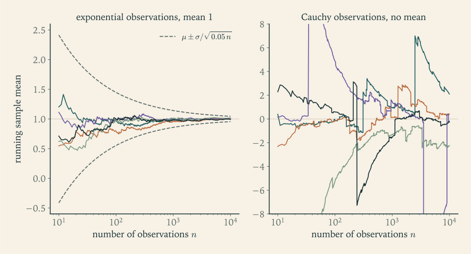
The weak law speaks about one sample size at a time. It says that for each large \(n\) , the average is probably close to \(\mu\) . It does not, by itself, say that a single infinite sequence of observations produces averages that converge. That is a stronger kind of convergence.
Definition 7.8 (almost sure convergence). A sequence \(Y_1,Y_2,\dots\) converges almost surely to \(c\) if
Almost sure convergence implies convergence in probability, and the converse is false; both facts are proved in Measure-Theoretic Probability. The left panel of Figure 7.1 suggests that sample means do converge in this stronger sense: each individual path enters the funnel and stays. Under a moment assumption this can be proved with the tools at hand. The key is a lemma about infinitely many events.
Lemma 7.9 (first Borel–Cantelli lemma). If \(A_1,A_2,\dots\) are events with \(\sum_{n=1}^{\infty}P(A_n)<\infty\) , then with probability one only finitely many of them occur.
Proof. If infinitely many of the \(A_n\) occur, then for every \(m\) at least one \(A_n\) with \(n\ge m\) occurs. So for every \(m\) the event “infinitely many occur” is contained in \(\bigcup_{n\ge m}A_n\) , whose probability is at most \(\sum_{n\ge m}P(A_n)\) by the countable union bound of Exercise 1.20. This is the tail of a convergent series and tends to \(0\) as \(m\to\infty\) . An event whose probability is at most every positive number has probability zero.
The lemma has a converse for independent events, which is the second Borel–Cantelli lemma (math.measure-theoretic-probability.borel-cantelli-lemmas); we shall not need it.
Theorem 7.10 (strong law of large numbers, fourth-moment case). Let \(X_1,X_2,\dots\) be independent and identically distributed with mean \(\mu\) and \(E[X_1^4]<\infty\) . Then \(\bar X_n\) converges almost surely to \(\mu\) .
Proof. Replacing \(X_i\) by \(X_i-\mu\) , assume \(\mu=0\) , and write \(S_n=X_1+\dots+X_n\) , \(\sigma^2=E[X_1^2]\) , and \(\kappa=E[X_1^4]\) . Expand \(S_n^4\) as a sum of products \(X_iX_jX_kX_l\) . By independence and \(E[X_i]=0\) , the expectation of a product vanishes whenever some index appears exactly once. The surviving terms are the \(n\) terms \(X_i^4\) , and the terms \(X_i^2X_j^2\) with \(i\ne j\) , each unordered pair arising in \(\binom42=6\) ways. So
using \(\sigma^4\le\kappa\) , which is Jensen’s inequality. Fix \(\varepsilon>0\) . By Markov’s inequality applied to \(S_n^4\) ,
These probabilities have a finite sum over \(n\) . By Lemma 7.9, with probability one \(\lvert\bar X_n\rvert\ge\varepsilon\) for only finitely many \(n\) . Apply this with \(\varepsilon=1/k\) for \(k=1,2,3,\dots\) The exceptional events have probability zero, and so does their countable union. Outside that union, for every \(k\) we have \(\lvert\bar X_n\rvert<1/k\) for all sufficiently large \(n\) , which says \(\bar X_n\to 0\) .
Compare the two proofs. The weak law used the second moment, and Chebyshev’s bound \(\sigma^2/(n\varepsilon^2)\) is not summable over \(n\) . The fourth moment gives a bound of order \(1/n^2\) , which is summable, and summability is what the Borel–Cantelli lemma converts into a statement about whole sequences.
The fourth-moment hypothesis is a convenience. Kolmogorov’s strong law states that for independent and identically distributed variables a finite mean alone suffices for almost sure convergence of the sample means (math.measure-theoretic-probability.strong-law-large-numbers). In applications the distinction between the two laws rarely matters. In interpretation it does: the strong law is what justifies speaking of the long-run average of a single unending series of trials.
The law of large numbers says where the sample mean goes. It says nothing about the shape of its fluctuations on the way. Those fluctuations are of size \(\sigma/\sqrt n\) , and after magnification by \(\sqrt n\) they turn out to follow a universal law.
Exercises
-
A nonnegative waiting time has mean \(4\) minutes. Give an upper bound for the probability that the wait is at least \(20\) minutes. Separately, examination scores have mean \(70\) and standard deviation \(10\) ; give a lower bound for the probability that a score lies strictly between \(50\) and \(90\) .
Answer
Markov: \(P(W\ge 20)\le 4/20=0.2\) . Chebyshev with \(k=2\) : \(P(\lvert X-70\rvert\ge 20)\le\tfrac14\) , so \(P(50<X<90)\ge\tfrac34\) .
-
For given numbers \(0<\mu<a\) , construct a nonnegative random variable with mean \(\mu\) for which Markov’s inequality at level \(a\) holds with equality, and show that if \(X\ge 0\) and \(P(X\ge a)=E[X]/a\) then \(X\) takes only the values \(0\) and \(a\) , with probability one.
Hint
Take \(X=a\) with probability \(\mu/a\) and \(X=0\) otherwise. For the second part, the proof of Theorem 7.1 shows \(E[X-a\mathbf 1_{\{X\ge a\}}]=0\) for a nonnegative variable \(X-a\mathbf 1_{\{X\ge a\}}\) ; a nonnegative variable with zero mean is zero with probability one, so \(X=a\mathbf 1_{\{X\ge a\}}\) .
-
Let \(X\) have mean \(\mu\) and variance \(\sigma^2\) , and let \(a>0\) . By applying Markov’s inequality to \((X-\mu+c)^2\) and choosing \(c\ge 0\) optimally, prove the one-sided inequality \(P(X-\mu\ge a)\le\dfrac{\sigma^2}{\sigma^2+a^2}\) , and evaluate the bound for the event of Example 7.3.
Solution
Let \(Y=X-\mu\) , with mean \(0\) and variance \(\sigma^2\) . For any \(c\ge 0\) , if \(Y\ge a\) then \(Y+c\ge a+c>0\) , so \((Y+c)^2\ge(a+c)^2\) . By Markov’s inequality applied to \((Y+c)^2\) ,
\[ P(Y\ge a)\le P\bigl((Y+c)^2\ge(a+c)^2\bigr)\le\frac{E[(Y+c)^2]}{(a+c)^2}=\frac{\sigma^2+c^2}{(a+c)^2}. \]Minimize over \(c\) . The derivative of the right-hand side has the sign of \(2c(a+c)-2(\sigma^2+c^2)=2(ca-\sigma^2)\) , so the minimum is at \(c=\sigma^2/a\) , where
\[ \frac{\sigma^2+\sigma^4/a^2}{(a+\sigma^2/a)^2}=\frac{\sigma^2(a^2+\sigma^2)/a^2}{(a^2+\sigma^2)^2/a^2}=\frac{\sigma^2}{\sigma^2+a^2}. \]This is the one-sided Chebyshev inequality, also called Cantelli’s inequality. For Example 7.3, \(\sigma^2=25\) and \(a=10\) give \(P(X\ge 60)\le\tfrac{25}{125}=0.2\) , a little better than the two-sided Chebyshev bound \(0.25\) , which wastes half of its allowance on the lower tail. The shift by \(c\) is what lets a one-sided event be bounded without controlling the other side.
-
For \(X\sim\mathrm{Exp}(1)\) and the event \(\{X\ge 5\}\) , compute Markov’s bound, Chebyshev’s bound, the optimized Chernoff bound, and the exact probability. Which of the bounds is best here, and what does that show about the claim that Chernoff bounds are always the sharpest?
Solution
Here \(\mu=1\) and \(\sigma^2=1\) .
Markov: \(P(X\ge 5)\le\tfrac15=0.2\) .
Chebyshev: \(\{X\ge 5\}\subseteq\{\lvert X-1\rvert\ge 4\}\) , so \(P(X\ge 5)\le\tfrac1{16}=0.0625\) .
Chernoff: \(M_X(t)=\tfrac{1}{1-t}\) for \(t<1\) , so the bound is \(e^{-5t}/(1-t)\) for \(0<t<1\) . Its logarithm \(-5t-\ln(1-t)\) has derivative \(-5+\tfrac1{1-t}\) , zero at \(t=\tfrac45\) . The optimized bound is \(5e^{-4}\approx 0.0916\) ; in general it is \(a\,e^{1-a}\) .
Exact: \(P(X\ge 5)=e^{-5}\approx 0.0067\) .
Chebyshev’s bound is the best of the three at this threshold. Chernoff’s bound decays exponentially in \(a\) and Chebyshev’s only like \(1/a^2\) , so Chernoff wins for large \(a\) (at \(a=6\) the two nearly tie, \(6e^{-5}\approx 0.040\) against \(\tfrac1{25}=0.04\) , and from \(a=7\) onward Chernoff is smaller), but not at every \(a\) . The claim “always sharpest” is false; each inequality is the best use of a particular piece of information, and the pieces are not nested.
-
Let \(X\sim\mathrm{Pois}(\lambda)\) and \(a>\lambda\) . Show that the optimized Chernoff bound is \(P(X\ge a)\le e^{-\lambda}\Bigl(\dfrac{e\lambda}{a}\Bigr)^{a}\) , and compare it with Chebyshev’s bound and the exact value when \(\lambda=10\) and \(a=20\) .
Solution
The Poisson moment generating function is \(M_X(t)=G_X(e^t)=\exp\bigl(\lambda(e^t-1)\bigr)\) . The logarithm of the Chernoff bound is
\[ -ta+\lambda(e^t-1), \]with derivative \(-a+\lambda e^t\) , which vanishes at \(e^t=a/\lambda\) . This \(t\) is positive because \(a>\lambda\) . Substituting \(t=\ln(a/\lambda)\) ,
\[ P(X\ge a)\le\exp\bigl(-a\ln(a/\lambda)+a-\lambda\bigr)=e^{-\lambda}\Bigl(\frac{e\lambda}{a}\Bigr)^{a}. \]For \(\lambda=10\) and \(a=20\) the bound is \(e^{-10}(e/2)^{20}\approx 0.0210\) . Chebyshev gives \(P(X\ge 20)\le P(\lvert X-10\rvert\ge 10)\le\tfrac{10}{100}=0.1\) , and the exact value is \(P(X\ge 20)\approx 0.0035\) . A deviation of \(10\) is more than three standard deviations, since \(\sigma=\sqrt{10}\approx 3.16\) , and at that distance the exponential bound is already five times better than Chebyshev’s, though still six times the truth.
-
Show that \(P(Z\ge a)\le e^{-a^2/2}\) for a standard normal variable \(Z\) and \(a>0\) , and compare the bound with the true probability at \(a=2\) and \(a=3\) .
Answer
\(M_Z(t)=e^{t^2/2}\) , so the bound is \(e^{-ta+t^2/2}\) , minimized at \(t=a\) , giving \(e^{-a^2/2}\) . At \(a=2\) : \(0.1353\) against the true \(0.0228\) . At \(a=3\) : \(0.0111\) against \(0.00135\) . The bound has the correct exponential rate and misses a factor of order \(1/a\) .
-
Use Jensen’s inequality to prove that \(E[\lvert X\rvert]\le\sqrt{E[X^2]}\) , and to prove the inequality between the arithmetic and geometric means of \(n\) positive numbers.
Solution
First inequality. The function \(\varphi(x)=x^2\) is convex. Apply Jensen’s inequality to the random variable \(\lvert X\rvert\) : \(\bigl(E[\lvert X\rvert]\bigr)^2\le E[\lvert X\rvert^2]=E[X^2]\) . Taking square roots gives \(E[\lvert X\rvert]\le\sqrt{E[X^2]}\) . (If \(E[X^2]=\infty\) there is nothing to prove.) Equivalently, the variance of \(\lvert X\rvert\) is nonnegative.
Means. Let \(x_1,\dots,x_n\) be positive numbers and let \(X\) be equally likely to be each of them. The logarithm is concave, since its second derivative \(-1/x^2\) is negative, so Jensen’s inequality in its concave form gives
\[ \frac1n\sum_{i=1}^{n}\ln x_i=E[\ln X]\le\ln E[X]=\ln\Bigl(\frac1n\sum_{i=1}^{n}x_i\Bigr). \]Exponentiating both sides, which preserves the inequality because the exponential is increasing,
\[ (x_1x_2\cdots x_n)^{1/n}\le\frac{x_1+\dots+x_n}{n}. \]The geometric mean is at most the arithmetic mean. Equality in Jensen’s inequality for a strictly concave function requires \(X\) to be constant, that is, all the \(x_i\) equal. Example 7.2 is the case \(n=2\) with the numbers \(1.5\) and \(0.6\) .
-
A journey of \(60\) kilometres is driven at a constant speed that is equally likely to be \(30\) or \(60\) kilometres per hour. A student computes the mean speed, \(45\) , and concludes that the mean journey time is \(60/45\) hours. Find the true mean journey time, identify the error, and say which direction of error Jensen’s inequality predicts.
Solution
The journey time is \(T=60/V\) . When \(V=30\) it is \(2\) hours and when \(V=60\) it is \(1\) hour, so
\[ E[T]=\tfrac12\cdot 2+\tfrac12\cdot 1=1.5\text{ hours}, \]not \(60/45\approx 1.33\) hours. The student computed \(60/E[V]\) in place of \(E[60/V]\) , moving the function \(v\mapsto 60/v\) through the expectation. That function is convex on \((0,\infty)\) , so Jensen’s inequality predicts \(E[60/V]\ge 60/E[V]\) : the naive calculation always underestimates the mean time, unless the speed is not random at all. Put differently, the speed that gives the correct mean time is the harmonic mean of the speeds, \(60/1.5=40\) kilometres per hour, which is less than their arithmetic mean \(45\) . A slow journey lasts longer, so slow speeds get more weight when averaging over time.
-
Use the weak law to find a number of rolls of a fair die that guarantees the sample mean lies within \(0.1\) of \(3.5\) with probability at least \(0.9\) .
Answer
One roll has variance \(\tfrac{35}{12}\) . The weak law requires \(\dfrac{35/12}{n\,(0.1)^2}\le 0.1\) , that is, \(n\ge 2917\) .
-
Let \(X_1,X_2,\dots\) be independent with common mean \(\mu\) and variances satisfying \(\operatorname{Var}(X_i)\le C\,i^{\alpha}\) for constants \(C\) and \(\alpha<1\) . Prove that the sample means converge in probability to \(\mu\) .
Hint
Independence gives \(\operatorname{Var}(\bar X_n)=n^{-2}\sum_{i\le n}\operatorname{Var}(X_i)\le Cn^{-2}\sum_{i\le n}i^{\alpha}\) . If \(\alpha\ge 0\) , each of the \(n\) terms \(i^{\alpha}\) is at most \(n^{\alpha}\) ; if \(\alpha<0\) , each is at most \(1\) . Either way the sum is at most \(n^{1+\max(\alpha,0)}\) , so \(\operatorname{Var}(\bar X_n)\le Cn^{\max(\alpha,0)-1}\) , which tends to zero because \(\alpha<1\) . Apply Chebyshev’s inequality to \(\bar X_n\) , whose mean is \(\mu\) . Note that the cruder bound \(Cn^{\alpha-1}\) is false for negative \(\alpha\) .
-
Let \(X_1,X_2,\dots\) have common mean \(\mu\) , common variance \(\sigma^2\) , and \(\operatorname{Cov}(X_i,X_j)=\sigma^2r^{\lvert i-j\rvert}\) for some \(0<r<1\) . Show that \(\operatorname{Var}(\bar X_n)\le\dfrac{\sigma^2}{n}\cdot\dfrac{1+r}{1-r}\) and deduce a weak law. Then show that if instead \(\operatorname{Cov}(X_i,X_j)=\sigma^2r\) for all \(i\ne j\) , the variance of \(\bar X_n\) does not tend to zero.
Solution
By Proposition 5.8(c),
\[ \operatorname{Var}(X_1+\dots+X_n)=\sum_{i=1}^{n}\sum_{j=1}^{n}\sigma^2r^{\lvert i-j\rvert}. \]For each fixed \(i\) , the inner sum over \(j\) is at most the sum over all integers \(d=j-i\) :
\[ \sum_{j=1}^{n}r^{\lvert i-j\rvert}\le 1+2\sum_{d=1}^{\infty}r^d=1+\frac{2r}{1-r}=\frac{1+r}{1-r}. \]Hence the variance of the sum is at most \(n\sigma^2\frac{1+r}{1-r}\) , and
\[ \operatorname{Var}(\bar X_n)\le\frac{\sigma^2}{n}\cdot\frac{1+r}{1-r}\longrightarrow 0 . \]Since \(E[\bar X_n]=\mu\) , Chebyshev’s inequality gives \(P(\lvert\bar X_n-\mu\rvert\ge\varepsilon)\le\frac{\sigma^2(1+r)}{n\varepsilon^2(1-r)}\to 0\) : a weak law holds. Positive correlation that decays geometrically costs a constant factor, as if the sample size were reduced from \(n\) to \(n\frac{1-r}{1+r}\) .
In the equicorrelated case, there are \(n\) variance terms and \(n(n-1)\) covariance terms, so
\[ \operatorname{Var}(\bar X_n)=\frac{n\sigma^2+n(n-1)\sigma^2r}{n^2}=\sigma^2\Bigl(r+\frac{1-r}{n}\Bigr)\longrightarrow\sigma^2r>0 . \]The variance of the average does not vanish, so no amount of averaging removes the common component. For instance, if \(X_i=W+V_i\) with a shared term \(W\) and independent terms \(V_i\) , the average converges to \(\mu+W-E[W]\) , which is random.
-
Prove that if \(Y_n\) converges in probability to \(c\) and \(g\) is a function continuous at \(c\) , then \(g(Y_n)\) converges in probability to \(g(c)\) .
Solution
Fix \(\varepsilon>0\) . Since \(g\) is continuous at \(c\) , there is \(\delta>0\) such that \(\lvert y-c\rvert<\delta\) implies \(\lvert g(y)-g(c)\rvert<\varepsilon\) . In contrapositive form: whenever \(\lvert g(y)-g(c)\rvert\ge\varepsilon\) , necessarily \(\lvert y-c\rvert\ge\delta\) . Applying this to \(y=Y_n\) at each outcome gives an inclusion of events,
\[ \{\lvert g(Y_n)-g(c)\rvert\ge\varepsilon\}\subseteq\{\lvert Y_n-c\rvert\ge\delta\}, \]and by monotonicity of probability
\[ P(\lvert g(Y_n)-g(c)\rvert\ge\varepsilon)\le P(\lvert Y_n-c\rvert\ge\delta)\longrightarrow 0, \]because \(Y_n\) converges in probability to \(c\) and \(\delta\) is a fixed positive number. Since \(\varepsilon\) was arbitrary, \(g(Y_n)\) converges in probability to \(g(c)\) . This is the step used in Example 7.6, with \(g\) the exponential function, to pass from the average of logarithms to the wealth itself.
-
Let \(Y_n\) equal \(n^2\) with probability \(1/n\) and \(0\) otherwise. Show that \(Y_n\) converges in probability to \(0\) while \(E[Y_n]\to\infty\) . Then prove that if \(E[Y_n]\to c\) and \(\operatorname{Var}(Y_n)\to 0\) , then \(Y_n\) converges in probability to \(c\) .
Answer
\(P(\lvert Y_n\rvert\ge\varepsilon)=1/n\to 0\) for every \(\varepsilon>0\) , while \(E[Y_n]=n^2\cdot\tfrac1n=n\to\infty\) . For the second part, \(E[(Y_n-c)^2]=\operatorname{Var}(Y_n)+(E[Y_n]-c)^2\to 0\) by Exercise 3.6, and Markov’s inequality applied to \((Y_n-c)^2\) gives \(P(\lvert Y_n-c\rvert\ge\varepsilon)\le E[(Y_n-c)^2]/\varepsilon^2\to 0\) .
-
The integral \(I=\int_0^1e^{-x^2}\,dx\) is estimated by the average of \(e^{-U_i^2}\) over \(n\) independent uniform variables \(U_i\) on \((0,1)\) . Given \(I\approx 0.7468\) and \(\int_0^1e^{-2x^2}\,dx\approx 0.5981\) , find the variance of one term and a sample size that guarantees an error of at most \(0.001\) with probability at least \(0.95\) .
Solution
Let \(g(u)=e^{-u^2}\) . By Theorem 4.5, \(E[g(U)]=\int_0^1e^{-x^2}dx=I\) , so the average \(\bar g_n\) of \(n\) independent copies has mean \(I\) , and by the weak law it converges in probability to \(I\) . The variance of one term is
\[ \operatorname{Var}(g(U))=E[g(U)^2]-I^2=\int_0^1e^{-2x^2}\,dx-I^2\approx 0.5981-0.7468^2\approx 0.0404 . \]Theorem 7.7 gives \(P(\lvert\bar g_n-I\rvert\ge 0.001)\le\dfrac{0.0404}{n\,(0.001)^2}\) , which is at most \(0.05\) when
\[ n\ge\frac{0.0404}{10^{-6}\cdot 0.05}\approx 808{,}000 . \]About eight hundred thousand evaluations guarantee three decimal places with probability \(0.95\) . As in Example 7.5, the cost is governed by the variance of a single term and by the square-root law, not by the smoothness of the integrand. Reducing the variance of the term, for example by subtracting from \(g\) a function with a known integral that resembles it, reduces the required \(n\) in proportion.
-
Use Proposition 7.5 to find a number of tosses of a fair coin that guarantees the proportion of heads is within \(0.05\) of \(\tfrac12\) with probability at least \(0.95\) , and compare with the number that Chebyshev’s inequality requires.
Answer
Proposition 7.5 needs \(2e^{-2n(0.05)^2}\le 0.05\) , that is, \(n\ge\ln 40/0.005\approx 737.8\) , so \(n=738\) . Chebyshev needs \(\dfrac{0.25}{n(0.05)^2}\le 0.05\) , that is, \(n=2000\) .
-
Let \(X_1,X_2,\dots\) be independent \(\mathrm{Exp}(1)\) variables. Use Lemma 7.9 to show that, with probability one, \(X_n>2\ln n\) for only finitely many \(n\) .
Hint
\(P(X_n>2\ln n)=e^{-2\ln n}=n^{-2}\) , and \(\sum n^{-2}<\infty\) . With \(\ln n\) in place of \(2\ln n\) the probabilities are \(1/n\) , whose sum diverges, and Lemma 7.9 gives no information.
-
For independent variables \(X_i\) taking the values \(-1\) and \(1\) with probability \(\tfrac12\) each, verify the formula \(E[S_n^4]=n\kappa+3n(n-1)\sigma^4\) of Theorem 7.10 in the case \(n=4\) by computing the distribution of \(S_4\) .
Solution
Here \(\sigma^2=E[X_i^2]=1\) and \(\kappa=E[X_i^4]=1\) , so the formula predicts \(E[S_4^4]=4\cdot 1+3\cdot 4\cdot 3\cdot 1=40\) .
Directly: \(S_4=2H-4\) , where \(H\sim\mathrm{Bin}(4,\tfrac12)\) is the number of plus signs. So \(S_4\) takes the values \(-4,-2,0,2,4\) with probabilities \(\tfrac1{16},\tfrac4{16},\tfrac6{16},\tfrac4{16},\tfrac1{16}\) , and
\[ E[S_4^4]=\frac{2\cdot 4^4+8\cdot 2^4+6\cdot 0}{16}=\frac{512+128}{16}=40 . \]The two agree. The structure of the count is visible in the number \(40=4+36\) : four terms of the form \(X_i^4\) , and for each of the \(\binom42=6\) pairs \(\{i,j\}\) , six arrangements of \(X_i^2X_j^2\) among the four factors. All other products contain some \(X_i\) to an odd power and average to zero.
-
In the setting of Example 7.2, suppose only a fixed fraction \(f\) of the wealth is exposed to the risky factor each year, the rest being held unchanged, so that the yearly factor is \(1+0.5f\) or \(1-0.4f\) . Find the fraction \(f\) that maximizes the expected logarithmic growth, and the resulting typical yearly growth factor.
Solution
The expected logarithmic growth per year when a fraction \(f\) is exposed is
\[ g(f)=\tfrac12\ln(1+0.5f)+\tfrac12\ln(1-0.4f),\qquad 0\le f\le 1 . \]Its derivative is \(g'(f)=\dfrac{0.25}{1+0.5f}-\dfrac{0.2}{1-0.4f}\) , which vanishes when \(0.25(1-0.4f)=0.2(1+0.5f)\) , that is, \(0.05=0.2f\) , so \(f=\tfrac14\) . The function \(g\) is concave, being a sum of logarithms of linear functions, so this is the maximum. There
\[ g\bigl(\tfrac14\bigr)=\tfrac12\ln(1.125\cdot 0.9)=\tfrac12\ln 1.0125\approx 0.0062, \]a typical yearly growth factor of \(\sqrt{1.0125}\approx 1.0062\) .
So the same risky opportunity that ruins an investor who stakes everything, \(g(1)\approx -0.0527\) , gives steady growth to one who stakes a quarter each year. By the weak law applied to the logarithms, as in Example 7.6, wealth with \(f=\tfrac14\) exceeds \(e^{0.005n}\) with probability tending to one. Expected wealth is maximized by \(f=1\) ; the probable outcome is maximized by a much smaller fraction.
-
The number of correct hats in the problem of Chapter 3 has mean \(1\) and variance \(1\) whenever there are at least two guests. Give the Markov and Chebyshev bounds for the probability that at least \(11\) guests receive their own hats, and explain why both bounds are valid for every such number of guests.
Answer
Markov: \(P(X\ge 11)\le\tfrac1{11}\approx 0.091\) . Chebyshev: \(P(X\ge 11)\le P(\lvert X-1\rvert\ge 10)\le\tfrac1{100}\) . Both hold for every number of guests from two upward because the mean and variance are \(1\) regardless of that number; the inequalities need nothing else. With a single guest the variance is \(0\) , not \(1\) , and with fewer than eleven guests the event is impossible, so the bounds are then true and uninformative.
-
Show that a sequence cannot converge in probability to two different constants.
Hint
If \(Y_n\) converged in probability to \(c\) and to \(c'\) with \(c\ne c'\) , take \(\varepsilon=\lvert c-c'\rvert/2\) . By the triangle inequality at least one of \(\lvert Y_n-c\rvert\ge\varepsilon\) and \(\lvert Y_n-c'\rvert\ge\varepsilon\) always holds, so the two probabilities sum to at least \(1\) and cannot both tend to \(0\) .