The law of large numbers says that the sample mean \(\bar X_n\) of independent observations approaches the mean \(\mu\) , the error being of the order of \(\sigma/\sqrt n\) . That is a statement about the size of the error. What about its shape? Divide the error by its own standard deviation,
and the result has mean \(0\) and variance \(1\) for every \(n\) : it neither collapses to a point nor escapes to infinity. Does its distribution settle down as \(n\) grows, and if so, to what?
One might expect the answer to depend on the distribution of the observations: skewed observations giving a skewed limit, discrete ones a discrete limit. It does not. Whatever the distribution of the summands, provided only that it has a finite variance, the distribution of \(Z_n\) approaches the same curve, the standard normal. Dice, coin tosses, exponential lifetimes, measurement errors: all are forgotten except for their mean and variance. This is the central limit theorem. It is the reason the normal distribution is ubiquitous, and it is the basis of nearly every large-sample approximation in applied probability and statistics.
8.1 Standardized sums and convergence in distribution
Throughout this chapter \(X_1,X_2,\dots\) are independent and identically distributed with mean \(\mu\) and variance \(\sigma^2\) , where \(0<\sigma^2<\infty\) ; \(S_n=X_1+\dots+X_n\) and \(\bar X_n=S_n/n\) .
Definition 8.1 (standardized sum). The standardized sum is
The two forms are equal, by dividing numerator and denominator of the first by \(n\) . Since \(E[S_n]=n\mu\) and \(\operatorname{Var}(S_n)=n\sigma^2\) , always \(E[Z_n]=0\) and \(\operatorname{Var}(Z_n)=1\) .
To say that the distribution of \(Z_n\) approaches a limit, we need a notion of convergence for distributions, as opposed to convergence of the random variables themselves.
Definition 8.2 (convergence in distribution). Random variables \(Y_n\) with distribution functions \(F_n\) converge in distribution to a random variable \(Y\) with distribution function \(F\) if
The restriction to continuity points is not a technical nuisance; without it the definition would give wrong answers in the simplest cases. Let \(Y_n\) be the constant \(1/n\) . Surely \(Y_n\) should converge to the constant \(0\) . The distribution function of \(Y_n\) is \(0\) to the left of \(1/n\) and \(1\) from \(1/n\) onward, so \(F_n(0)=0\) for every \(n\) , while the distribution function of the constant \(0\) has \(F(0)=1\) . Convergence fails at \(x=0\) , which is exactly the point where \(F\) jumps, and holds everywhere else. When the limit distribution function is continuous everywhere, as \(\Phi\) is, the exception never arises and convergence in distribution means \(F_n(x)\to F(x)\) for all \(x\) . It then follows that \(P(a<Y_n\le b)\to F(b)-F(a)\) for all \(a<b\) .
Convergence in distribution involves only the distributions of the \(Y_n\) , not how they are related to one another as functions on a sample space. It is the weakest of the three modes of convergence in this book: convergence in probability implies it, and for a constant limit the two are equivalent.
Example 8.1: Watching skewness disappear
Let the \(X_i\) be exponential with rate \(1\) , so that \(\mu=\sigma=1\) . By Corollary 5.14(d), \(S_n\) has the gamma density with shape \(n\) , and so the distribution of \(Z_n=(S_n-n)/\sqrt n\) can be computed exactly for every \(n\) . Three probabilities tell the story.
| \(n\) | \(P(Z_n\le -1)\) | \(P(Z_n\le 0)\) | \(P(Z_n\le 1)\) |
|---|---|---|---|
| \(1\) | \(0\) | \(0.632\) | \(0.865\) |
| \(5\) | \(0.147\) | \(0.560\) | \(0.847\) |
| \(30\) | \(0.157\) | \(0.524\) | \(0.843\) |
| \(100\) | \(0.158\) | \(0.513\) | \(0.842\) |
| limit | \(0.159\) | \(0.500\) | \(0.841\) |
The last row holds the values \(\Phi(-1)\) , \(\Phi(0)\) , and \(\Phi(1)\) . For \(n=1\) the standardized variable is \(X_1-1\) , which cannot be below \(-1\) at all and is below its mean with probability \(1-e^{-1}\approx 0.632\) : a single exponential variable is strongly skewed. By \(n=30\) the three probabilities are within \(0.025\) of their limits, and by \(n=100\) within \(0.014\) . The slowest to converge is the middle column, which measures the asymmetry directly.
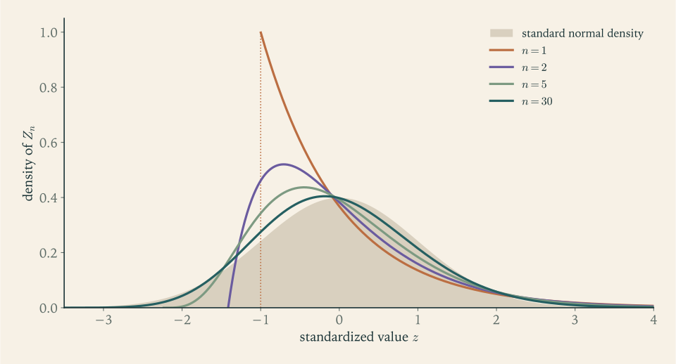
Figure 8.1 shows the densities behind the table. Two features deserve attention. The approach to the normal curve is not uniform across the range: the centre settles first, while the left tail, where the exponential sums have a hard lower limit, lags. And the convergence is of distributions, not of the summands: each \(X_i\) remains as skewed as ever.
8.2 The theorem and its proof
Theorem 8.3 (central limit theorem). Let \(X_1,X_2,\dots\) be independent and identically distributed with mean \(\mu\) and finite variance \(\sigma^2>0\) . Then the standardized sums converge in distribution to the standard normal distribution:
We prove the theorem under one additional hypothesis, that the moment generating function of the \(X_i\) exists in the sense of Definition 4.14. The proof needs two auxiliary facts. The first is a limit from calculus.
Lemma 8.4 (the exponential limit). If \(a_n\to a\) , then \(\bigl(1+\tfrac{a_n}{n}\bigr)^n\to e^{a}\) .
Proof. For \(\lvert u\rvert\le\tfrac12\) the series \(\ln(1+u)=u-\tfrac{u^2}{2}+\tfrac{u^3}{3}-\cdots\) gives \(\lvert\ln(1+u)-u\rvert\le\tfrac{u^2}{2}\bigl(1+\lvert u\rvert+\lvert u\rvert^2+\cdots\bigr)\le u^2\) . Since \(a_n\) is bounded, \(u_n=a_n/n\) satisfies \(\lvert u_n\rvert\le\tfrac12\) for large \(n\) , and then \(\bigl\lvert n\ln(1+u_n)-a_n\bigr\rvert\le n\,u_n^2=a_n^2/n\to 0\) . So \(n\ln(1+a_n/n)\to a\) , and the exponential function is continuous.
The second fact is the bridge from transforms to distributions. Theorem 4.16 said that a moment generating function determines a distribution. The following strengthening says that the correspondence is continuous.
Theorem 8.5 (continuity theorem for moment generating functions). Let \(Y_n\) and \(Y\) be random variables whose moment generating functions are finite on a common open interval containing \(0\) . If \(M_{Y_n}(t)\to M_Y(t)\) for every \(t\) in that interval, then \(Y_n\) converges in distribution to \(Y\) .
The proof belongs to Measure-Theoretic Probability, where the result is established for the characteristic function \(E[e^{itX}]\)
, a transform that is finite for every random variable (math.measure-theoretic-probability.levy-continuity-theorem).
Proof of Theorem 8.3, assuming the moment generating function exists. Let \(Y_i=(X_i-\mu)/\sigma\) . The \(Y_i\) are independent and identically distributed with mean \(0\) and variance \(1\) , and by Proposition 4.17 their common moment generating function \(M\) is finite on an interval \((-\delta,\delta)\) . The standardized sum is \(Z_n=(Y_1+\dots+Y_n)/\sqrt n\) , so by Theorem 5.13 and Proposition 4.17,
By Theorem 4.15, \(M\) is given near \(0\) by its power series, whose first three coefficients are \(1\) , \(E[Y_1]=0\) , and \(E[Y_1^2]/2=\tfrac12\) . Hence
Fix a real number \(t\) and put \(s=t/\sqrt n\) , which tends to \(0\) :
By Lemma 8.4, \(M_{Z_n}(t)\to e^{t^2/2}\) , which is the moment generating function of \(N(0,1)\) by Example 4.9. This holds for every real \(t\) . To apply Theorem 8.5 we need one open interval around \(0\) on which all the functions involved are finite, and \((-\delta,\delta)\) is such an interval: it is contained in \((-\delta\sqrt n,\delta\sqrt n)\) , where \(M_{Z_n}\) is finite, for every \(n\ge 1\) , and \(e^{t^2/2}\) is finite everywhere. Theorem 8.5 therefore gives convergence in distribution. Since \(\Phi\) is continuous, the convergence holds at every \(x\) .
Look at what the proof used. Independence turned the transform of the sum into a product. Identical distribution made the product an \(n\) -th power. The mean was removed by centring, the variance fixed the coefficient of \(s^2\) , and every higher moment was swept into the remainder \(r(s)\) , which the scaling by \(\sqrt n\) sends to zero. That is the mechanism of universality: after standardization, only the first two moments survive the limit.
The additional hypothesis is not needed for the theorem. Replacing \(M(t)\)
by the characteristic function throughout, the same computation works with nothing assumed beyond a finite variance; that is the form in which the theorem is proved in Measure-Theoretic Probability (math.measure-theoretic-probability.lindeberg-levy-clt). The hypothesis that cannot be dropped is the finite variance itself, as Section 8.5 shows.
There is also a way to see why the limit, if there is one, must be normal. Split a sum of \(2n\) terms into two halves. The standardized sum of all \(2n\) terms is \((Z_n'+Z_n'')/\sqrt2\) , where \(Z_n'\) and \(Z_n''\) are independent standardized sums of \(n\) terms. If the distributions converge to a limit law, that law must be reproduced when two independent copies are added and divided by \(\sqrt2\) . By Corollary 5.14 the standard normal law has this property, and it can be shown to be the only law with mean \(0\) and variance \(1\) that does.
8.3 Normal approximation in practice
For calculation, the theorem is used in the form: for large \(n\) ,
The word “approximately” refers to probabilities of intervals. The recipe is to standardize the endpoint and read \(\Phi\) .
Example 8.2: Waiting for fifty customers
Service times are independent and exponential with mean \(2\) minutes, so each has standard deviation \(2\) as well. The total time \(S\) to serve \(50\) customers has mean \(100\) and standard deviation \(2\sqrt{50}\approx 14.14\) minutes. The probability that it exceeds two hours is approximately
Here the exact answer is available, because \(S\) has a gamma distribution: \(P(S>120)\approx 0.0844\) . The approximation is in error by about \(0.006\) , on the low side, because the exponential distribution is skewed to the right and with \(50\) terms some of that skewness remains, fattening the right tail.
When the \(X_i\) are integer-valued, so is \(S_n\) , and its distribution function is a staircase that the smooth curve \(\Phi\) cuts through. The fit is much improved by treating each integer \(k\) as the interval from \(k-\tfrac12\) to \(k+\tfrac12\) .
Definition 8.6 (continuity correction). For an integer-valued sum \(S_n\) and integers \(j\le k\) , the normal approximation with continuity correction is
In particular \(P(S_n\ge k)\) is approximated using the endpoint \(k-\tfrac12\) , and \(P(S_n\le k)\) using \(k+\tfrac12\) .
Example 8.3: Binomial probabilities three ways
Let \(X\sim\mathrm{Bin}(100,\tfrac12)\) , a sum of \(100\) fair indicators, with mean \(50\) and standard deviation \(5\) .
A central interval. The exact value of \(P(45\le X\le 55)\) is \(0.7287\) . Without the correction, standardizing \(45\) and \(55\) gives \(\Phi(1)-\Phi(-1)\approx 0.6827\) , which is poor: it leaves out half of the probability of each endpoint. With the correction the endpoints are \(44.5\) and \(55.5\) , and
correct to four places.
A tail. Example 7.3 bounded \(P(X\ge 60)\) by \(0.25\) with Chebyshev’s inequality and by \(0.1335\) with Chernoff’s, the exact value being \(0.0284\) . The corrected normal approximation uses the endpoint \(59.5\) :
The approximation is within \(0.0003\) of the truth, incomparably closer than either bound. The price is that it is not a bound: nothing in the central limit theorem, as stated, says on which side of the truth the approximation lies or how far away it may be.
Example 8.4: One hundred dice, and the questions of Chapter 7
Dice. One roll of a fair die has mean \(3.5\) and variance \(\tfrac{35}{12}\) . The total \(S\) of \(100\) rolls has mean \(350\) and standard deviation \(\sqrt{100\cdot 35/12}\approx 17.08\) . With the continuity correction,
The exact value, obtained by convolving the distribution of one die with itself a hundred times, is \(0.1269\) .
The opening question of Chapter 7. For \(10{,}000\) tosses of a fair coin the number of heads has mean \(5000\) and standard deviation \(50\) . The event that the proportion differs from \(\tfrac12\) by \(0.01\) or more is \(\lvert X-5000\rvert\ge 100\) , and with the correction
which agrees with the exact value \(0.0466\) to four places. Chebyshev’s guarantee was \(0.25\) .
The sample size of Example 7.4. For the relative frequency in \(n\) trials to lie within \(0.05\) of \(p\) with probability about \(0.95\) , we need \(0.05\) to be about \(1.96\) standard deviations of the relative frequency, since \(\Phi(1.96)=0.975\) . The standard deviation is \(\sqrt{p(1-p)/n}\le\tfrac{1}{2\sqrt n}\) , so it suffices that
so \(385\) trials. Chebyshev’s inequality demanded \(2000\) and Hoeffding’s \(738\) . Those were guarantees; this is an approximation whose accuracy at \(n=385\) is good for \(p\) near \(\tfrac12\) and deteriorates as \(p\) approaches \(0\) or \(1\) .
Statements of this kind, about how close a relative frequency is likely to be to a known \(p\)
, are probability statements. Turning them around, into statements about an unknown \(p\)
given an observed frequency, is the theory of confidence intervals in Mathematical Statistics (math.mathematical-statistics.confidence-sets).
8.4 How good is the approximation?
The central limit theorem is a statement about a limit. For a particular \(n\) it promises nothing. A quantitative companion fills the gap.
Theorem 8.7 (Berry–Esseen bound). Let \(X_1,X_2,\dots\) be independent and identically distributed with mean \(\mu\) , variance \(\sigma^2>0\) , and finite third absolute central moment \(\gamma=E[\lvert X_1-\mu\rvert^3]\) . Then for every \(n\) and every real \(x\) ,
where \(C\) is an absolute constant, known to be smaller than \(0.48\) .
We do not prove this theorem. It makes three things precise. The error is of order \(1/\sqrt n\) , no better in general. The constant in front depends on the summand distribution only through the ratio \(\gamma/\sigma^3\) , which is large for strongly skewed or heavy-tailed summands. And the bound is uniform in \(x\) and absolute: it controls the difference of probabilities, not their ratio.
For a fair coin, \(\lvert X_1-\tfrac12\rvert=\tfrac12\) always, so \(\gamma/\sigma^3=1\) and the bound for \(n=100\) is \(0.048\) . The true maximal error of the uncorrected approximation is about \(0.040\) , half the probability of the most likely value, so the bound is nearly attained; it is the continuity correction that removes most of this error. For an indicator with success probability \(p\) the ratio is \((p^2+q^2)/\sqrt{pq}\) , which grows without bound as \(p\to 0\) .
Example 8.5: Rare events, where the normal curve is the wrong tool
Return to Example 3.6: \(X\sim\mathrm{Bin}(1000,0.002)\) , with mean \(2\) and standard deviation \(\sqrt{1.996}\approx 1.413\) . Here \(n\) is large, and the normal approximation is still poor, because the summands are extremely skewed: the Berry–Esseen bound is about \(0.34\) , useless.
| Probability | Exact | Normal with correction | Poisson |
|---|---|---|---|
| \(P(X=0)\) | \(0.1351\) | \(0.1442\) | \(0.1353\) |
| \(P(X\ge 7)\) | \(0.0045\) | \(0.0007\) | \(0.0045\) |
For \(P(X=0)\) the normal value \(\Phi\bigl(\tfrac{0.5-2}{1.413}\bigr)=\Phi(-1.062)\) is off by \(0.009\) , tolerable in absolute terms. For the upper tail \(P(X\ge 7)\) the normal value \(1-\Phi(3.185)\) is too small by a factor of six. The Poisson approximation of Theorem 3.12 is accurate to the digits shown in both cases.
The lesson is about which limit theorem fits which regime. With \(n\) large and \(p\) fixed, the binomial is close to normal; a common working rule asks for both \(np\) and \(n(1-p)\) to be at least \(10\) . With \(n\) large and \(np\) moderate, it is close to Poisson. The count of failures here has mean \(2\) ; it is a small-number phenomenon however many trials produced it.
Common mistake. Trusting the normal approximation far out in the tails. The central limit theorem controls absolute errors, and in the far tails the probabilities themselves are tiny, so a small absolute error can be an enormous relative error. In Example 8.2 the exact probability of exceeding the mean by four standard deviations is several times the normal value; in Example 8.5 the factor was six at about three standard deviations. For tail probabilities many standard deviations out, the exponential bounds of Section 7.3, which capture the correct rate of decay, are the better guide, and for rare-event counts the Poisson approximation is. The normal approximation is a description of the centre of the distribution, within two or three standard deviations of the mean.
8.5 What the theorem does not say
The central limit theorem is so widely quoted that its misreadings are as common as its uses. Five limits on its meaning follow.
It does not say that the observations are normal, or become normal. The \(X_i\) keep whatever distribution they have. A thousand exponential lifetimes have a histogram that looks exponential. It is their sum, or their mean, that is approximately normal.
It requires a finite variance. For independent Cauchy variables the sample mean has the same Cauchy distribution as a single observation, for every \(n\) , as noted in Section 7.5. No scaling makes the sum normal. More generally, for summands whose tail probabilities \(P(\lvert X\rvert>x)\) decay like a power \(x^{-\alpha}\) with \(0<\alpha<2\) , properly scaled sums converge to non-normal limits, the stable laws, and the scaling is not \(\sqrt n\) . The boundary case \(\alpha=2\) is different: the variance is still infinite, yet the limit is normal, with a scaling slightly larger than \(\sqrt n\) .
It requires independence, or something close to it. Suppose \(X_i=W+V_i\) , where \(W\) is a random variable shared by all the terms and the \(V_i\) are independent of each other and of \(W\) . The shared term is not averaged away, as Exercise 7.11 showed, and the sum is dominated by \(nW\) , whose distribution is whatever the distribution of \(W\) is. Versions of the theorem do exist for weakly dependent sequences, and for independent summands that are not identically distributed provided no single one dominates; each has its own hypotheses, which must be checked.
It concerns a fixed distribution as the number of terms grows. If the distribution of the summands changes with \(n\) , the conclusion can change, as the Poisson limit shows: there the success probability shrinks as \(n\) grows, and the limit is not normal.
It describes fluctuations on one particular scale. The law of large numbers and the central limit theorem are statements about the same sum at different magnifications.
| Law of large numbers | Central limit theorem | |
|---|---|---|
| Quantity | \(\bar X_n-\mu\) | \(\sqrt n\,(\bar X_n-\mu)/\sigma\) |
| Limit | the constant \(0\) | the \(N(0,1)\) distribution |
| Mode of convergence | in probability, or almost surely | in distribution |
| Moment needed | finite mean | finite variance |
| Typical use | the average is near \(\mu\) | how near, with what probability |
On the scale of \(n\) , deviations of the sum are negligible: \(P(\lvert S_n-n\mu\rvert\ge\varepsilon n)\to 0\) . On the scale of \(\sqrt n\) they have a nondegenerate limit: \(P(\lvert S_n-n\mu\rvert\ge c\,\sigma\sqrt n)\to 2\bigl(1-\Phi(c)\bigr)\) . On any fixed scale they are unbounded: \(P(\lvert S_n-n\mu\rvert\ge c)\to 1\) for every constant \(c\) . Knowing which scale a question lives on is the first step in answering it.
Two closure properties noted earlier now appear as instances of the theorem. A \(\mathrm{Pois}(n)\) variable is a sum of \(n\) independent \(\mathrm{Pois}(1)\) variables, and a gamma variable with shape \(n\) is a sum of \(n\) independent exponentials, by Corollary 5.14. So Poisson distributions with large mean and gamma distributions with large shape are approximately normal, without further proof.
The course ends here, at the two limit theorems on which the applications of probability rest. Three directions lead on. Mathematical Statistics reverses the viewpoint, reasoning from observed averages back to unknown parameters, with the central limit theorem supplying the error distributions. Stochastic Processes studies random quantities that evolve in time; there the standardized sums of this chapter, viewed as functions of time, converge to Brownian motion. And Measure-Theoretic Probability rebuilds the foundations, so that expectation, conditional expectation, and the modes of convergence are defined once for all random variables, and the theorems quoted without proof in this book are proved.
Exercises
-
Independent quantities each have mean \(5\) and standard deviation \(2\) . For \(64\) of them, use the central limit theorem to approximate the probability that their sum exceeds \(340\) and the probability that their mean lies between \(4.5\) and \(5.5\) .
Answer
The sum has mean \(320\) and standard deviation \(2\sqrt{64}=16\) , so \(P(S>340)\approx 1-\Phi(1.25)\approx 0.106\) . The mean has standard deviation \(2/8=0.25\) , so \(P(4.5<\bar X<5.5)\approx 2\Phi(2)-1\approx 0.954\) .
-
Let \(X\sim\mathrm{Bin}(400,0.2)\) . Approximate \(P(X\le 70)\) with and without the continuity correction, and compare both with the exact value \(0.1164\) .
Solution
The mean is \(np=80\) and the standard deviation is \(\sqrt{400\cdot 0.2\cdot 0.8}=8\) .
Without the correction, standardize \(70\) : \(z=(70-80)/8=-1.25\) , giving \(\Phi(-1.25)\approx 0.1056\) .
With the correction, the event \(\{X\le 70\}\) is treated as \(\{X\le 70.5\}\) : \(z=(70.5-80)/8=-1.1875\) , giving \(\Phi(-1.1875)\approx 0.1175\) .
The exact value is \(0.1164\) . The uncorrected approximation is off by about \(0.011\) and the corrected one by about \(0.001\) . The correction matters because a single value near the boundary carries appreciable probability: \(P(X=70)\approx 0.023\) , and stopping the normal area at \(70\) instead of \(70.5\) discards about half of it. For a binomial variable with standard deviation \(8\) , each integer spans one eighth of a standard deviation, which is not negligible on the scale of \(\Phi\) .
-
A fair die is rolled \(30\) times. Use the normal approximation with continuity correction to estimate the probability that the total lies between \(95\) and \(115\) inclusive.
Answer
The total has mean \(105\) and standard deviation \(\sqrt{30\cdot 35/12}\approx 9.354\) . With endpoints \(94.5\) and \(115.5\) , \(z=\pm 10.5/9.354=\pm 1.1225\) , and the probability is approximately \(2\Phi(1.1225)-1\approx 0.738\) . The exact value is \(0.737\) .
-
A proportion is to be estimated by the relative frequency in \(n\) independent trials. Find the \(n\) suggested by the central limit theorem for the relative frequency to lie within \(0.03\) of the true proportion with probability about \(0.95\) , find the \(n\) guaranteed by Chebyshev’s inequality for the same requirement, and state precisely the difference in the status of the two answers.
Solution
Central limit theorem. The relative frequency \(\hat p\) has mean \(p\) and standard deviation \(\sqrt{p(1-p)/n}\le\tfrac{1}{2\sqrt n}\) , and is approximately normal. It lies within \(1.96\) standard deviations of \(p\) with probability about \(0.95\) . So the requirement is met, approximately, when \(1.96\cdot\tfrac{1}{2\sqrt n}\le 0.03\) :
\[ n\ge\Bigl(\frac{1.96}{0.06}\Bigr)^2\approx 1067.1,\qquad\text{so } n=1068 . \]Chebyshev. The guarantee \(P(\lvert\hat p-p\rvert\ge 0.03)\le\dfrac{1/4}{n\,(0.03)^2}\le 0.05\) requires
\[ n\ge\frac{0.25}{0.0009\cdot 0.05}\approx 5556 . \]Status. The Chebyshev figure is a guarantee: for every \(p\) and for that \(n\) , the probability of a miss is at most \(0.05\) , with no approximation involved. The central limit figure is an approximation: at \(n=1068\) the probability of a miss is close to \(0.05\) when \(p\) is near \(\tfrac12\) (and smaller for other \(p\) , because the bound \(p(1-p)\le\tfrac14\) is then generous), but the theorem itself supplies no error bound. The factor of about five between the two sample sizes is the price of the guarantee. This is the calculation behind the familiar statement that a poll of about a thousand people has a margin of error of three percentage points.
-
Let \(Y_n\) be uniformly distributed on the \(n\) points \(\tfrac1n,\tfrac2n,\dots,\tfrac nn\) . Prove from Definition 8.2 that \(Y_n\) converges in distribution to a \(\mathrm{Unif}(0,1)\) variable, although every \(Y_n\) is discrete and the limit is continuous.
Solution
The distribution function of \(Y_n\) at \(x\in[0,1]\) counts the points \(k/n\) not exceeding \(x\) :
\[ F_n(x)=\frac{\lfloor nx\rfloor}{n}, \]where \(\lfloor nx\rfloor\) is the integer part of \(nx\) ; also \(F_n(x)=0\) for \(x<0\) and \(F_n(x)=1\) for \(x\ge 1\) . Since \(nx-1<\lfloor nx\rfloor\le nx\) ,
\[ x-\frac1n<F_n(x)\le x, \]so \(F_n(x)\to x\) for every \(x\in[0,1]\) . The limit function, \(0\) for \(x<0\) , \(x\) on \([0,1]\) , and \(1\) for \(x>1\) , is the distribution function \(F\) of \(\mathrm{Unif}(0,1)\) , which is continuous everywhere, so convergence at every point is exactly what Definition 8.2 requires.
Each \(Y_n\) is discrete, with \(P(Y_n=k/n)=1/n\) , and the limit has no atoms. There is no contradiction: convergence in distribution compares distribution functions, and a staircase with \(n\) steps of height \(1/n\) is uniformly within \(1/n\) of the straight line. The individual masses \(1/n\) tend to zero. This is the same phenomenon as in the central limit theorem for coin tossing, where discrete binomial distributions converge to the continuous normal law.
-
Let \(Y_n\) be the constant \(-\tfrac1n\) and \(Y_n'\) the constant \(\tfrac1n\) . For each sequence, find \(\lim F_n(0)\) and compare it with the distribution function of the constant \(0\) at \(0\) . What does the comparison show about the restriction to continuity points in Definition 8.2?
Answer
For \(Y_n=-\tfrac1n\) : \(F_n(0)=1\) for all \(n\) , equal to \(F(0)=1\) . For \(Y_n'=\tfrac1n\) : \(F_n(0)=0\) for all \(n\) , so the limit is \(0\ne F(0)\) . Both sequences obviously approach \(0\) , and both converge in distribution to \(0\) under Definition 8.2, because \(0\) is the one point where \(F\) is discontinuous and is exempt. Requiring convergence at every point would wrongly reject the second sequence.
-
Let \(N_\lambda\sim\mathrm{Pois}(\lambda)\) . Compute the moment generating function of \((N_\lambda-\lambda)/\sqrt\lambda\) and show that it converges to \(e^{t^2/2}\) as \(\lambda\to\infty\) , for every real \(t\) . What does Theorem 8.5 then say?
Solution
By Proposition 4.17 with \(a=1/\sqrt\lambda\) and \(b=-\sqrt\lambda\) , and the Poisson moment generating function \(\exp(\lambda(e^t-1))\) ,
\[ M_\lambda(t)=E\Bigl[\exp\Bigl(t\,\frac{N_\lambda-\lambda}{\sqrt\lambda}\Bigr)\Bigr]=\exp\Bigl(-t\sqrt\lambda+\lambda\bigl(e^{t/\sqrt\lambda}-1\bigr)\Bigr). \]Expand the inner exponential: \(e^{u}-1=u+\tfrac12u^2+u^2\,r(u)\) with \(r(u)\to 0\) as \(u\to 0\) . With \(u=t/\sqrt\lambda\) ,
\[ \lambda\bigl(e^{t/\sqrt\lambda}-1\bigr)=t\sqrt\lambda+\tfrac12t^2+t^2\,r\bigl(t/\sqrt\lambda\bigr). \]The term \(t\sqrt\lambda\) cancels, leaving the exponent \(\tfrac12t^2+t^2r(t/\sqrt\lambda)\to\tfrac12t^2\) as \(\lambda\to\infty\) . Hence \(M_\lambda(t)\to e^{t^2/2}\) for every real \(t\) .
All these functions are finite for all \(t\) , and the limit is the moment generating function of \(N(0,1)\) . Theorem 8.5 therefore says that \((N_\lambda-\lambda)/\sqrt\lambda\) converges in distribution to the standard normal law: a Poisson variable with large mean is approximately \(N(\lambda,\lambda)\) . For integer \(\lambda\) this also follows from the central limit theorem and Corollary 5.14(b); the transform argument covers all real \(\lambda\) at once.
-
Use the normal approximation with continuity correction to estimate \(P(N\ge 120)\) for \(N\sim\mathrm{Pois}(100)\) , and compare with the exact value \(0.0282\) .
Answer
Mean \(100\) , standard deviation \(10\) , corrected endpoint \(119.5\) : \(1-\Phi(1.95)\approx 0.0256\) , against the exact \(0.0282\) . The normal value is somewhat low, since the Poisson distribution is skewed to the right.
-
An analyst says: “We have a thousand independent exponential lifetimes with mean \(1\) . By the central limit theorem the data are approximately normal, so about \(68\) percent of the lifetimes lie within one standard deviation of the mean.” Find the true proportion, explain what the central limit theorem does say about these data, and give a correct statement involving \(68\) percent.
Solution
For an exponential distribution with mean \(1\) the standard deviation is also \(1\) , so “within one standard deviation of the mean” is the interval \((0,2)\) , and the proportion of lifetimes in it is close to
\[ P(0<X<2)=1-e^{-2}\approx 0.865, \]not \(0.68\) . The data are a sample from the exponential distribution, and by the law of large numbers their histogram resembles the exponential density, however many there are. Collecting more data makes the histogram a better picture of the exponential curve, not a more normal one.
What the central limit theorem says concerns the sample mean of the thousand lifetimes: it is approximately normal with mean \(1\) and standard deviation \(1/\sqrt{1000}\approx 0.032\) . A correct statement with \(68\) percent: if the experiment of collecting a thousand lifetimes and averaging them were repeated many times, about \(68\) percent of the averages would fall between \(0.968\) and \(1.032\) .
The analyst confused the distribution of the observations with the distribution of their mean. The figure \(68\) percent belongs to the normal law, and the normal law describes the average.
-
The sum of \(36\) independent exponential variables with rate \(3\) has mean \(12\) and standard deviation \(2\) . Approximate the probability that it exceeds \(16\) , and compare with the exact gamma value \(0.0309\) . In which direction is the error, and why?
Answer
\(z=(16-12)/2=2\) , so the approximation is \(1-\Phi(2)\approx 0.0228\) , below the exact \(0.0309\) . The summands are skewed to the right, and with \(36\) terms the sum retains some of that skewness, which thickens the upper tail beyond two standard deviations and thins the lower one.
-
Forty-eight numbers are each rounded to the nearest integer, and the rounding errors are modelled as independent and uniform on \((-\tfrac12,\tfrac12)\) . Approximate the probability that the error in the sum exceeds \(3\) in absolute value.
Solution
Each rounding error is uniform on an interval of length \(1\) , so it has mean \(0\) and variance \(\tfrac1{12}\) . The error \(E\) in the sum of \(48\) numbers is the sum of the \(48\) independent errors, with mean \(0\) and variance \(48/12=4\) , so its standard deviation is \(2\) . By the central limit theorem \(E/2\) is approximately standard normal, and
\[ P(\lvert E\rvert>3)\approx 2\bigl(1-\Phi(1.5)\bigr)\approx 0.1336 . \]No continuity correction is needed, because the summands are continuous. The approximation is very good here: the exact value, from the piecewise polynomial distribution of a sum of uniform variables, is \(0.1339\) . Uniform summands are symmetric and bounded, so the third-moment term that governs the leading error vanishes and convergence is fast.
The result illustrates the square-root law in a practical setting. The worst possible error in the sum is \(24\) , but errors of that size require all \(48\) roundings to go the same way; the typical error is about \(2\) .
-
For a fair coin and \(n=100\) , evaluate the Berry–Esseen bound with \(C=0.48\) , and compare it with the largest difference between the binomial distribution function and its uncorrected normal approximation, which occurs at the mean and equals half of \(P(X=50)\approx 0.0796\) .
Solution
For a fair coin indicator, \(\sigma=\tfrac12\) and \(\lvert X_1-\tfrac12\rvert=\tfrac12\) with probability one, so \(\gamma=\tfrac18\) and \(\gamma/\sigma^3=1\) . The Berry–Esseen bound with \(C=0.48\) and \(n=100\) is
\[ \frac{0.48\cdot 1}{\sqrt{100}}=0.048 . \]The binomial distribution function jumps at each integer, while \(\Phi\) is continuous. At the mean, \(x=50\) , the symmetric binomial distribution has \(P(X\le 50)=\tfrac12+\tfrac12P(X=50)\) , whereas the uncorrected normal approximation gives \(\Phi(0)=\tfrac12\) . The difference is \(\tfrac12P(X=50)\approx 0.0398\) , and this is the largest discrepancy over all \(x\) .
So the actual maximal error, \(0.040\) , is about five sixths of the bound \(0.048\) . The bound is close to sharp in this case, and the error it describes is almost entirely the discreteness error that the continuity correction removes: with the correction, the approximation at \(50\) becomes \(\Phi(0.1)\approx 0.5398\) , equal to the exact value to four places.
-
For \(X\sim\mathrm{Bin}(500,0.004)\) compare the exact value of \(P(X=0)\) with its Poisson approximation and its normal approximation with continuity correction, and say which limit theorem applies and why.
Answer
Exact: \(0.996^{500}\approx 0.1348\) . Poisson with mean \(2\) : \(e^{-2}\approx 0.1353\) . Normal with correction: \(\Phi\bigl((0.5-2)/\sqrt{1.992}\bigr)=\Phi(-1.063)\approx 0.1439\) . The Poisson limit applies: \(n\) is large, \(p\) is small, and \(np=2\) is far below the size needed for a normal approximation.
-
Use the central limit theorem to prove the weak law of large numbers for independent and identically distributed variables with finite variance, without using Chebyshev’s inequality.
Solution
Fix \(\varepsilon>0\) . In terms of the standardized sum,
\[ P(\lvert\bar X_n-\mu\rvert<\varepsilon)=P\Bigl(\lvert Z_n\rvert<\frac{\varepsilon\sqrt n}{\sigma}\Bigr). \]Let \(c>0\) be arbitrary. Once \(n\) is large enough that \(\varepsilon\sqrt n/\sigma>c\) , the event \(\{-c<Z_n\le c\}\) is contained in the event above, so
\[ P(\lvert\bar X_n-\mu\rvert<\varepsilon)\ge P(-c<Z_n\le c). \]By the central limit theorem, applied at the two points \(c\) and \(-c\) , the right-hand side tends to \(\Phi(c)-\Phi(-c)=2\Phi(c)-1\) . So for every \(c\) , the probabilities \(P(\lvert\bar X_n-\mu\rvert<\varepsilon)\) are eventually larger than any number below \(2\Phi(c)-1\) . Since \(2\Phi(c)-1\to 1\) as \(c\to\infty\) , and probabilities never exceed \(1\) , it follows that \(P(\lvert\bar X_n-\mu\rvert<\varepsilon)\to 1\) , which is the weak law.
The argument shows that the central limit theorem is the finer statement: it describes the distribution of the error on the scale \(1/\sqrt n\) , and any fixed tolerance \(\varepsilon\) eventually corresponds to arbitrarily many standard deviations.
-
Let \(X_i=W+V_i\) , where \(W,V_1,V_2,\dots\) are independent, \(W\) takes the values \(-1\) and \(1\) with probability \(\tfrac12\) each, and the \(V_i\) are standard normal. Find the exact distribution of \(\bar X_n\) and its limit as \(n\to\infty\) , and explain which hypothesis of Theorem 8.3 fails.
Solution
The sample mean is \(\bar X_n=W+\bar V_n\) , where \(\bar V_n\) , the mean of \(n\) independent standard normal variables, is \(N(0,1/n)\) by Corollary 5.14(a) and is independent of \(W\) . Conditioning on \(W\) ,
\[ P(\bar X_n\le x)=\tfrac12\,\Phi\bigl(\sqrt n\,(x+1)\bigr)+\tfrac12\,\Phi\bigl(\sqrt n\,(x-1)\bigr). \]So \(\bar X_n\) is an equal mixture of \(N(-1,1/n)\) and \(N(1,1/n)\) . As \(n\to\infty\) the first term tends to \(\tfrac12\) for \(x>-1\) and to \(0\) for \(x<-1\) , and the second tends to \(\tfrac12\) for \(x>1\) and to \(0\) for \(x<1\) . The limit is the distribution function of \(W\) : \(0\) below \(-1\) , \(\tfrac12\) between \(-1\) and \(1\) , and \(1\) above \(1\) . Thus \(\bar X_n\) converges in distribution to \(W\) , a random limit, not to the mean \(E[X_i]=0\) ; and no normal limit arises for the standardized sum, which is \(\sqrt{n/2}\,W\) plus a term whose distribution does not depend on \(n\) , and so diverges.
The hypothesis that fails is independence. Each \(X_i\) has mean \(0\) and variance \(2\) , and the \(X_i\) are identically distributed, but \(\operatorname{Cov}(X_i,X_j)=\operatorname{Var}(W)=1\) for \(i\ne j\) . This is the equicorrelated case of Exercise 7.11: averaging removes the individual terms \(V_i\) and leaves the shared term untouched.
-
A classical recipe for generating an approximately standard normal number is to add twelve independent \(\mathrm{Unif}(0,1)\) numbers and subtract \(6\) . Verify that the result has mean \(0\) and variance \(1\) , state its range, and compare the normal value of \(P(\lvert Z\rvert>2)\) with the exact value \(0.0446\) for the recipe.
Answer
Each uniform has mean \(\tfrac12\) and variance \(\tfrac1{12}\) , so the sum of twelve has mean \(6\) and variance \(1\) ; subtracting \(6\) gives mean \(0\) and variance \(1\) . The range is \([-6,6]\) , so values beyond six standard deviations are impossible. Normal: \(P(\lvert Z\rvert>2)\approx 0.0455\) ; the recipe gives \(0.0446\) , slightly lighter tails.
-
An insurer holds \(10{,}000\) independent policies. Each produces a claim with probability \(0.01\) , and a claim, when it occurs, has mean \(5\) and standard deviation \(5\) , in thousands. Find the mean and variance of the payout on one policy, and use the central limit theorem to find the reserve that covers the total payout with probability \(0.99\) .
Solution
One policy. Let \(I\) indicate a claim, \(P(I=1)=0.01\) , and let the payout be \(Y\) , equal to the claim size when \(I=1\) and \(0\) otherwise. Conditioning on \(I\) : \(E[Y\mid I]=5I\) and \(\operatorname{Var}(Y\mid I)=25I\) . By the tower property and the law of total variance,
\[ E[Y]=5\cdot 0.01=0.05,\qquad \operatorname{Var}(Y)=25\cdot 0.01+25\cdot 0.01\cdot 0.99=0.25+0.2475=0.4975 . \]The portfolio. The total payout \(S\) of \(10{,}000\) independent policies has mean \(500\) and variance \(4975\) , so its standard deviation is \(\sqrt{4975}\approx 70.5\) . By the central limit theorem \(S\) is approximately normal. The reserve \(r\) with \(P(S\le r)=0.99\) satisfies \((r-500)/70.5\approx 2.326\) , the \(0.99\) quantile of the standard normal law, so
\[ r\approx 500+2.326\cdot 70.5\approx 664 , \]in thousands. A reserve of about a third more than the expected payout suffices with probability \(0.99\) .
Two cautions. The individual payouts are extremely skewed, being zero \(99\) percent of the time, so the normal approximation is less accurate than the large number of policies suggests; the expected number of claims, \(100\) , is the effective sample size. To see the size of the effect, suppose claim sizes are exponential with mean \(5\) , which has the required standard deviation. Then the total is a binomial mixture of gamma variables and can be computed exactly: a reserve of \(664\) covers it with probability about \(0.986\) , and the exact \(0.99\) reserve is about \(675\) . The normal approximation is slightly optimistic in the upper tail, as it was in Example 8.2. And the calculation depends on independence: a common cause that affects many policies at once would add a term that does not average out.
-
Let the \(X_i\) have finite third moment and skewness \(\kappa_3=E[(X_1-\mu)^3]/\sigma^3\) . Show that \(E[Z_n^3]=\kappa_3/\sqrt n\) , and relate this to the rate in Theorem 8.7 and to the middle column of the table in Example 8.1.
Hint
With \(Y_i=(X_i-\mu)/\sigma\) , expand \(\bigl(\sum Y_i\bigr)^3\) ; by independence and \(E[Y_i]=0\) only the \(n\) terms \(Y_i^3\) survive, so \(E[Z_n^3]=n\kappa_3/n^{3/2}\) . Skewness decays at the rate \(1/\sqrt n\) , the rate in the Berry–Esseen bound, and it shows up in the table as the slow drift of \(P(Z_n\le 0)\) toward \(\tfrac12\) .
-
In Example 7.6, the wealth after \(100\) years is at least \(1\) exactly when the number of good years is at least \(56\) . Approximate that probability by the normal approximation with continuity correction and compare with the exact value \(0.1356\) .
Answer
The number of good years is \(\mathrm{Bin}(100,\tfrac12)\) with mean \(50\) and standard deviation \(5\) . \(P(K\ge 56)\approx 1-\Phi\bigl(\tfrac{55.5-50}{5}\bigr)=1-\Phi(1.1)\approx 0.1357\) , against the exact \(0.1356\) .
-
Let \(S_n\) be the number of heads in \(n\) tosses of a fair coin. Find the limits, as \(n\to\infty\) , of \(P(\lvert S_n-\tfrac n2\rvert<10)\) , of \(P(\lvert S_n-\tfrac n2\rvert<\sqrt n)\) , and of \(P(\lvert S_n-\tfrac n2\rvert<0.01n)\) , justifying each.
Solution
\(S_n\) has mean \(n/2\) and standard deviation \(\sqrt n/2\) ; write \(Z_n=(S_n-n/2)/(\sqrt n/2)\) .
Fixed width. \(\{\lvert S_n-\tfrac n2\rvert<10\}=\{\lvert Z_n\rvert<20/\sqrt n\}\) . For any \(c>0\) this event is contained in \(\{\lvert Z_n\rvert<c\}\) once \(20/\sqrt n\le c\) , so its probability is eventually at most \(P(\lvert Z_n\rvert<c)\to 2\Phi(c)-1\) . Since \(c\) can be taken arbitrarily small and \(2\Phi(c)-1\to 0\) as \(c\to 0\) , the limit is \(0\) . A window of fixed width captures a vanishing share of a distribution whose spread grows like \(\sqrt n\) .
Width proportional to the square root of the number of tosses. \(\{\lvert S_n-\tfrac n2\rvert<\sqrt n\}=\{\lvert Z_n\rvert<2\}\) , and by the central limit theorem the probability tends to \(2\Phi(2)-1\approx 0.9545\) .
Width proportional to the number of tosses. \(\{\lvert S_n-\tfrac n2\rvert<0.01n\}=\{\lvert S_n/n-\tfrac12\rvert<0.01\}\) , whose probability tends to \(1\) by the weak law of large numbers.
The three limits, \(0\) , \(0.9545\) , and \(1\) , are the three regimes described at the end of Section 8.5: on a fixed scale the deviation is certain to be large, on the scale \(\sqrt n\) it has a normal limit, and on the scale \(n\) it is negligible.