Consider two random variables \(X\) and \(Y\) , each equal to \(0\) or \(1\) with probability \(\tfrac12\) . What is the variance of \(X+Y\) ?
The question cannot be answered. If \(X\) and \(Y\) come from two separate tosses of a fair coin, the sum takes the values \(0,1,2\) with probabilities \(\tfrac14,\tfrac12,\tfrac14\) and its variance is \(\tfrac12\) . If \(Y\) is the same toss as \(X\) , the sum is \(0\) or \(2\) and its variance is \(1\) . If \(Y=1-X\) , the sum is always \(1\) and its variance is \(0\) . In all three cases \(X\) and \(Y\) have exactly the same individual distributions. What differs is how they behave together, and no amount of information about each one separately can supply that.
This chapter studies distributions of pairs. It defines the joint law and shows how the individual and conditional laws are extracted from it; makes independence of random variables precise; introduces covariance, the single number that settles the variance of a sum; and finds the distribution of a sum of independent variables, first by convolution and then, much more easily, by generating functions.
5.1 Joint mass functions and marginals
Definition 5.1 (joint and marginal mass functions). The joint probability mass function of discrete random variables \(X\) and \(Y\) defined on the same probability space is
The marginal mass functions are those of \(X\) and \(Y\) individually, and they are recovered by summing out the other variable:
The summation formula is additivity over the partition of \(\{X=x\}\) by the values of \(Y\) ; it was already used in the proof of Theorem 3.5. The name comes from the habit of writing a joint mass function as a table and its row and column sums in the margins. The joint law determines the marginals, and the opening paragraph shows that the marginals do not determine the joint law.
Example 5.1: Two counts that share a toss
Toss a fair coin three times. Let \(X\) be the number of heads among the first two tosses and \(Y\) the number among the last two. The eight equally likely outcomes give the joint table below; for instance \((X,Y)=(1,1)\) arises from HTH and THT.
| \(Y=0\) | \(Y=1\) | \(Y=2\) | \(p_X\) | |
|---|---|---|---|---|
| \(X=0\) | \(\tfrac18\) | \(\tfrac18\) | \(0\) | \(\tfrac14\) |
| \(X=1\) | \(\tfrac18\) | \(\tfrac28\) | \(\tfrac18\) | \(\tfrac12\) |
| \(X=2\) | \(0\) | \(\tfrac18\) | \(\tfrac18\) | \(\tfrac14\) |
| \(p_Y\) | \(\tfrac14\) | \(\tfrac12\) | \(\tfrac14\) | \(1\) |
Each marginal is \(\mathrm{Bin}(2,\tfrac12)\) , as it must be. The two zeros in the table record that \(X\) and \(Y\) cannot differ by two, since they share the middle toss. Any expectation involving both variables is a sum over the table; for example
Since \(E[X]E[Y]=1\) , the product does not have the product of the means as its mean. We return to this table twice below.
5.2 Joint densities
Definition 5.2 (joint density). Random variables \(X\) and \(Y\) are jointly continuous with joint density \(f_{X,Y}\) if \(f_{X,Y}\) is a nonnegative integrable function on the plane such that
for every region \(A\) of the plane for which the integral is defined.
Probability is now volume under a surface. The total volume is one, and any curve, having zero area, has probability zero; in particular \(P(X=Y)=0\)
for jointly continuous variables. Double integrals are computed as iterated integrals in either order, by Fubini’s theorem (math.multivariable-calculus.fubini-continuous). Taking \(A\)
to be the half-plane to the left of the vertical line at \(x\)
shows that \(X\)
has a density, obtained by integrating out \(y\)
:
Expectations are computed by the two-variable form of Theorem 4.5,
valid whenever the integral converges absolutely. With \(g(x,y)=ax+by\) this formula gives linearity of expectation for jointly continuous variables in one line, by splitting the integral and integrating out one variable in each piece.
Example 5.2: A density on the unit square
Let \(f(x,y)=x+y\) for \(0<x<1\) , \(0<y<1\) , and \(0\) elsewhere. It is nonnegative and
The marginal density of \(X\) is \(f_X(x)=\int_0^1(x+y)\,dy=x+\tfrac12\) for \(0<x<1\) , and by symmetry \(f_Y(y)=y+\tfrac12\) . To find \(P(X+Y\le 1)\) , integrate over the triangle below the diagonal:
The triangle is half the square but has only a third of the probability, because the density is larger toward the corner \((1,1)\) . The limits of the inner integral depend on the outer variable; setting them correctly, from a sketch of the region, is most of the work in problems of this kind.
Example 5.3: A density on a triangle
Let \((X,Y)\) be uniformly distributed on the triangle \(0<x<y<1\) . The triangle has area \(\tfrac12\) , so the joint density is \(2\) on it and \(0\) elsewhere. For \(0<x<1\) the possible values of \(y\) run from \(x\) to \(1\) , and for \(0<y<1\) the possible values of \(x\) run from \(0\) to \(y\) :
The joint density is constant, yet neither marginal is uniform: small values of \(x\) are compatible with many values of \(y\) and large ones with few. This joint law arises naturally. If two independent points are chosen uniformly in \((0,1)\) , the smaller and the larger of them have exactly this distribution, since each unordered pair corresponds to two equally weighted ordered pairs.
5.3 Conditional distributions
For discrete variables conditioning needs nothing new: for each \(x\) with \(p_X(x)>0\) the conditional mass function of \(Y\) given \(X=x\) is
It is the row of the joint table at \(x\) , divided by its row sum. In Example 5.1, given \(X=1\) the conditional masses of \(Y\) are \(\tfrac14,\tfrac12,\tfrac14\) ; given \(X=2\) they are \(0,\tfrac12,\tfrac12\) .
For continuous variables the event \(\{X=x\}\) has probability zero and Definition 2.1 does not apply. The definition is made by analogy and justified by a limit.
Definition 5.3 (conditional density). Let \(X\) and \(Y\) have joint density \(f_{X,Y}\) . For each \(x\) with \(f_X(x)>0\) , the conditional density of \(Y\) given \(X=x\) is
Conditional probabilities given \(X=x\) are defined by \(P(Y\in B\mid X=x)=\int_B f_{Y\mid X}(y\mid x)\,dy\) .
For fixed \(x\) this is a genuine density in \(y\) : it is nonnegative and its integral is \(f_X(x)/f_X(x)=1\) . To see that it deserves its name, condition on the event that \(X\) lies in a short interval, which has positive probability. Where the densities are continuous,
after dividing the numerator and the denominator by \(h\) . Geometrically, the conditional density is the profile of the joint density along the vertical line at \(x\) , rescaled to have area one.
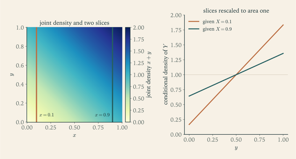
For the density of Example 5.2, the slices are
Figure 5.1 shows two of them. Along \(x=0.1\) the conditional density rises from \(\tfrac16\) to \(\tfrac{11}{6}\) ; along \(x=0.9\) it rises only from \(\tfrac{9}{14}\) to \(\tfrac{19}{14}\) . A small value of \(X\) makes large values of \(Y\) relatively more likely than a large value of \(X\) does. If the renormalized slices were all the same curve, knowing \(X\) would tell us nothing about \(Y\) ; that situation is independence, defined in the next section.
Definition 5.3 rearranges into a multiplication rule, \(f_{X,Y}(x,y)=f_X(x)\,f_{Y\mid X}(y\mid x)\) , and integrating over \(x\) gives continuous versions of the two theorems of Chapter 2:
The first is the law of total probability and the second is Bayes’ rule, with sums replaced by integrals.
Example 5.4: Building a joint law from a conditional one
In Example 5.3, dividing the joint density \(2\) by \(f_X(x)=2(1-x)\) gives \(f_{Y\mid X}(y\mid x)=\dfrac{1}{1-x}\) for \(x<y<1\) : given the smaller point, the larger is uniform on what remains of the interval. Likewise, given \(Y=y\) , \(X\) is uniform on \((0,y)\) .
The multiplication rule is more often used in the other direction, to specify a model in stages. Break a stick of unit length at a uniformly random point and keep the left piece, of length \(X\sim\mathrm{Unif}(0,1)\) . Then break that piece at a uniformly random point and keep its left piece, of length \(Y\) . The second stage says that, given \(X=x\) , \(Y\sim\mathrm{Unif}(0,x)\) . Hence
and the marginal density of the final piece is
This is a legitimate density, unbounded near \(0\) , with \(\int_0^1(-\ln y)\,dy=1\) . The final piece is very likely to be short: its density is largest where \(y\) is smallest.
5.4 Independent random variables
Definition 5.4 (independent random variables). Random variables \(X\) and \(Y\) are independent if
for all sets \(A\) and \(B\) of real numbers for which these probabilities are defined. Random variables \(X_1,\dots,X_n\) are mutually independent if \(P(X_1\in A_1,\dots,X_n\in A_n)=\prod_i P(X_i\in A_i)\) for all such sets, and an infinite sequence is independent if every finite subcollection is. Variables that are mutually independent and have a common distribution are called independent and identically distributed.
In words, every event that concerns \(X\) alone is independent, in the sense of Definition 2.8, of every event that concerns \(Y\) alone. The definition is unwieldy to check directly, and in practice one uses a criterion in terms of mass functions or densities.
Proposition 5.5 (factorization criterion). Discrete random variables \(X\) and \(Y\) are independent if and only if \(p_{X,Y}(x,y)=p_X(x)\,p_Y(y)\) for all \(x\) and \(y\) . Jointly continuous random variables are independent if and only if the product \(f_X(x)f_Y(y)\) is a joint density for them. More generally, if a joint mass function or joint density can be written as \(g(x)\,h(y)\) for all real \(x\) and \(y\) , then \(X\) and \(Y\) are independent.
Proof. In the discrete case, take \(A=\{x\}\) and \(B=\{y\}\) to see that independence implies factorization. Conversely, if the mass function factorizes, then
In the continuous case, if \(f_Xf_Y\) is a joint density, the same computation with integrals in place of sums gives independence. Conversely, if \(X\) and \(Y\) are independent then \(P(X\le x,Y\le y)=F_X(x)F_Y(y)=\int_{-\infty}^{x}\int_{-\infty}^{y}f_X(s)f_Y(t)\,dt\,ds\) , so integrating \(f_Xf_Y\) over any quadrant gives the probability that \((X,Y)\) lies in that quadrant. Definition 5.2 asks for the same identity over every region, and passing from quadrants to all regions is a uniqueness fact about measures: two probability laws on the plane that agree on every quadrant agree on every region. We quote that fact without proof; it belongs to Measure-Theoretic Probability. Granting it, \(f_Xf_Y\) is a joint density. For the last statement, integrate or sum \(g(x)h(y)\) over \(y\) : the marginal of \(X\) is \(g(x)\) times the constant \(c=\int h\) or \(\sum h\) , likewise the marginal of \(Y\) is \(h(y)\) times \(\int g\) or \(\sum g\) , and the product of the two constants is the total mass, \(1\) ; so \(p_Xp_Y\) or \(f_Xf_Y\) equals \(gh\) .
The phrase “for all real \(x\) and \(y\) ” hides a condition on the support. A joint density that factorizes on a region that is not a rectangle with sides parallel to the axes does not factorize on the whole plane, because the indicator of the region is part of the formula. In Example 5.3 the density is the constant \(2\) on the triangle, which looks like a product, and yet \(X\) and \(Y\) are dependent: the possible values of \(Y\) depend on \(X\) . A support that is not a product set is an immediate proof of dependence. On the unit square, the density \(4xy\) factorizes, so its coordinates are independent; the density \(x+y\) of Example 5.2 does not factorize, and Figure 5.1 has already shown the dependence. In Example 5.1, \(p_{X,Y}(0,2)=0\) while \(p_X(0)\,p_Y(2)=\tfrac1{16}\) , so those two counts are dependent.
Two consequences of independence are used constantly. First, functions of independent random variables are independent: if \(X\) and \(Y\) are independent, so are \(g(X)\) and \(h(Y)\) , because \(\{g(X)\in A\}\) is the event \(\{X\in g^{-1}(A)\}\) , which concerns \(X\) alone. Second, expectations of products factorize.
Theorem 5.6 (expectation of a product). If \(X\) and \(Y\) are independent, and \(g\) and \(h\) are functions with \(E[\lvert g(X)\rvert]<\infty\) and \(E[\lvert h(Y)\rvert]<\infty\) , then
Proof. We prove the theorem when \(X\) and \(Y\) are both discrete and when they are jointly continuous. In the discrete case, by the two-variable form of Theorem 3.4 and Proposition 5.5,
the double series being absolutely convergent because the corresponding identity for \(\lvert g\rvert\) and \(\lvert h\rvert\) shows it has a finite sum of absolute values. The jointly continuous case is identical with integrals.
The theorem is true for every pair of independent random variables, and it will be used in that generality, in particular when one variable is discrete and the other continuous. The two computations above do not reach that case, because such a pair has neither a joint mass function nor a joint density. The general statement is quoted from Measure-Theoretic Probability, where independence is shown to mean that the joint law is the product of the two marginal laws, and the product formula then follows from Tonelli’s theorem (math.measure-theoretic-probability.independence-product-law).
5.5 Covariance and correlation
Definition 5.7 (covariance). For random variables \(X\) and \(Y\) with finite variances and means \(\mu_X\) and \(\mu_Y\) , the covariance is
The second form follows by expanding the product and using linearity. Covariance is positive when \(X\) and \(Y\) tend to be on the same side of their means at the same time and negative when they tend to be on opposite sides.
Proposition 5.8 (algebra of covariance). For random variables with finite variances and constants \(a,b,c\) :
(a) \(\operatorname{Cov}(X,Y)=\operatorname{Cov}(Y,X)\) , \(\operatorname{Cov}(X,X)=\operatorname{Var}(X)\) , and \(\operatorname{Cov}(X,c)=0\) ;
(b) \(\operatorname{Cov}(aX+bY,Z)=a\operatorname{Cov}(X,Z)+b\operatorname{Cov}(Y,Z)\) , and similarly in the second argument;
(c) for any \(X_1,\dots,X_n\) ,
Proof. Part (a) is immediate from the definition. For (b), the deviation of \(aX+bY\) from its mean is \(a(X-\mu_X)+b(Y-\mu_Y)\) ; multiply by \(Z-\mu_Z\) and take expectations. For (c), by (a) and (b) the variance of the sum is \(\operatorname{Cov}\bigl(\sum_iX_i,\sum_jX_j\bigr)=\sum_i\sum_j\operatorname{Cov}(X_i,X_j)\) ; the \(n\) terms with \(i=j\) are the variances, and the remaining terms come in equal pairs.
Part (c) is the formula that the opening question was missing. For two variables it reads \(\operatorname{Var}(X+Y)=\operatorname{Var}(X)+\operatorname{Var}(Y)+2\operatorname{Cov}(X,Y)\) . In the three versions of that question the covariances are \(0\) , \(\tfrac14\) , and \(-\tfrac14\) , giving variances \(\tfrac12\) , \(1\) , and \(0\) .
Theorem 5.9 (independent variables are uncorrelated). If \(X\) and \(Y\) are independent with finite variances, then \(\operatorname{Cov}(X,Y)=0\) . Consequently, if \(X_1,\dots,X_n\) are pairwise independent with finite variances,
Proof. By Theorem 5.6 with \(g\) and \(h\) the identity, \(E[XY]=E[X]E[Y]\) . The second statement is Proposition 5.8(c) with every covariance zero.
Variances of independent variables add; standard deviations do not. For independent and identically distributed \(X_1,\dots,X_n\) with variance \(\sigma^2\) , the sum has variance \(n\sigma^2\) and standard deviation \(\sigma\sqrt n\) , and the sample mean \(\bar X_n=(X_1+\dots+X_n)/n\) has
This square-root law is the quantitative heart of Chapters 7 and 8: to halve the spread of an average, one needs four times as many observations.
Variables with zero covariance are called uncorrelated. Theorem 5.9 says that independence implies zero covariance. The converse is false.
Example 5.5: Uncorrelated and completely dependent
Let \(X\) take the values \(-1\) , \(0\) , \(1\) with probability \(\tfrac13\) each, and let \(Y=X^2\) . Then \(E[X]=0\) and \(E[XY]=E[X^3]=0\) , so
Yet \(Y\) is a function of \(X\) , the strongest possible dependence, and the product rule fails visibly: \(P(X=0,Y=0)=\tfrac13\) , while \(P(X=0)P(Y=0)=\tfrac13\cdot\tfrac13=\tfrac19\) .
The covariance vanishes because the dependence is symmetric: large positive and large negative values of \(X\) both go with large \(Y\) , and their contributions cancel. Covariance detects only the tendency of two variables to increase together along a straight line.
To compare strengths of association, covariance must be freed of units.
Definition 5.10 (correlation). If \(X\) and \(Y\) have finite positive variances, their correlation coefficient is
Theorem 5.11 (Cauchy–Schwarz inequality for covariance). If \(X\) and \(Y\) have finite positive variances, then \(-1\le\rho(X,Y)\le 1\) , that is, \(\lvert\operatorname{Cov}(X,Y)\rvert\le\sigma_X\sigma_Y\) . Moreover \(\rho=1\) or \(\rho=-1\) if and only if \(Y=a+bX\) with probability one for some constants \(a\) and \(b\ne 0\) , and then \(\rho\) has the sign of \(b\) .
Proof. Let \(\tilde X=(X-\mu_X)/\sigma_X\) and \(\tilde Y=(Y-\mu_Y)/\sigma_Y\) . Each has mean \(0\) and variance \(1\) , and \(\operatorname{Cov}(\tilde X,\tilde Y)=\rho\) by Proposition 5.8(b). By part (c) of that proposition,
The plus sign gives \(\rho\ge -1\) and the minus sign gives \(\rho\le 1\) . If \(\rho=1\) , then \(\operatorname{Var}(\tilde X-\tilde Y)=0\) , so by Proposition 3.9 the variable \(\tilde X-\tilde Y\) equals its mean \(0\) with probability one, which says \(Y=\mu_Y+\tfrac{\sigma_Y}{\sigma_X}(X-\mu_X)\) ; similarly \(\rho=-1\) gives a linear relation with negative slope. Conversely, if \(Y=a+bX\) then \(\operatorname{Cov}(X,Y)=b\,\sigma_X^2\) and \(\sigma_Y=\lvert b\rvert\sigma_X\) , so \(\rho=b/\lvert b\rvert\) .
Example 5.6: Two correlations
The shared toss. In Example 5.1, \(E[XY]=\tfrac54\) and both means are \(1\) , so \(\operatorname{Cov}(X,Y)=\tfrac14\) . Each variable is \(\mathrm{Bin}(2,\tfrac12)\) with variance \(\tfrac12\) , so
The value has a transparent meaning. Write \(X=T_1+T_2\) and \(Y=T_2+T_3\) with \(T_i\) the indicators of heads on the three tosses. By bilinearity and independence of the tosses, \(\operatorname{Cov}(X,Y)=\operatorname{Var}(T_2)=\tfrac14\) : the covariance is the variance of the part they share.
The density on the unit square. For Example 5.2, \(E[X]=\int_0^1x\bigl(x+\tfrac12\bigr)dx=\tfrac7{12}\) , \(E[X^2]=\int_0^1x^2\bigl(x+\tfrac12\bigr)dx=\tfrac5{12}\) , and
Hence \(\operatorname{Var}(X)=\tfrac5{12}-\tfrac{49}{144}=\tfrac{11}{144}\) and \(\operatorname{Cov}(X,Y)=\tfrac13-\tfrac{49}{144}=-\tfrac1{144}\) , so \(\rho=-\tfrac1{11}\) . The dependence visible in Figure 5.1 is real and weak, and it is negative, as the slices suggested.
Example 5.7: The variance of a hypergeometric count
A sample of \(n\) items is drawn without replacement from a population of \(N\) items, of which \(K\) are marked; let \(p=K/N\) . Section 3.5 found the mean \(np\) of the number \(X\) of marked items in the sample. For the variance, write \(X=I_1+\dots+I_n\) with \(I_i\) the indicator that the \(i\) -th draw is marked. Each \(I_i\) has variance \(p(1-p)\) . For \(i\ne j\) , both draws are marked with probability \(\frac KN\cdot\frac{K-1}{N-1}\) , so
after a line of algebra. The covariance is negative: a marked item drawn early leaves fewer for later. Proposition 5.8(c), with \(n(n-1)\) ordered pairs, gives
This is the binomial variance multiplied by the finite-population correction \((N-n)/(N-1)\) . For the number of hearts in a five-card hand, \(p=\tfrac14\) and the variance is \(\tfrac{15}{16}\cdot\tfrac{47}{51}=\tfrac{235}{272}\approx 0.864\) , against \(0.9375\) for five draws with replacement. When \(n=N\) the correction is zero, as it should be: sampling the whole population leaves nothing to chance.
5.6 Sums of independent random variables
Theorem 5.12 (convolution). Let \(X\) and \(Y\) be independent. If they are discrete, then
If they have densities \(f_X\) and \(f_Y\) , then \(X+Y\) has density
Proof. In the discrete case, partition \(\{X+Y=z\}\) by the value of \(X\) and use independence: \(P(X=x,Y=z-x)=p_X(x)p_Y(z-x)\) . In the continuous case the joint density is \(f_X(x)f_Y(y)\) , and substituting \(y=u-x\) in the inner integral,
where the order of integration was exchanged in the last step. The inner function of \(u\) is therefore a density for \(X+Y\) .
Example 5.8: Two convolutions
Two uniform variables. Let \(X\) and \(Y\) be independent and \(\mathrm{Unif}(0,1)\) . The integrand \(f_X(x)f_Y(z-x)\) equals \(1\) when \(0<x<1\) and \(0<z-x<1\) , that is, when \(\max(0,z-1)<x<\min(1,z)\) . The length of that interval is the density:
The sum of two flat densities is a triangle peaked at \(1\) . The whole difficulty is in the limits of integration, which change form at \(z=1\) .
Two exponential variables. Let \(X\) and \(Y\) be independent and \(\mathrm{Exp}(\lambda)\) . The integrand is nonzero for \(0<x<z\) , and
The wait for the second of two successive exponential events is no longer memoryless; its density vanishes at \(0\) , since two events cannot both occur at once.
Convolution integrals quickly become laborious. Generating functions replace them by multiplication.
Theorem 5.13 (generating functions of independent sums). Let \(X\) and \(Y\) be independent. Then
for every \(t\) at which both factors are finite. If \(X\) and \(Y\) take values in the nonnegative integers, then \(G_{X+Y}(s)=G_X(s)\,G_Y(s)\) for \(\lvert s\rvert\le 1\) . Both statements extend to any finite number of mutually independent variables.
Proof. Apply Theorem 5.6 with \(g(x)=e^{tx}\) and \(h(y)=e^{ty}\) : \(E[e^{t(X+Y)}]=E[e^{tX}e^{tY}]=E[e^{tX}]\,E[e^{tY}]\) . For the second statement use \(g(x)=s^x\) and \(h(y)=s^y\) .
Combined with the uniqueness theorems, Theorem 3.14(a) and Theorem 4.16, this identifies the distributions of sums at sight.
Corollary 5.14 (closure under independent sums). Let the random variables in each statement be mutually independent.
(a) If \(X_i\sim N(\mu_i,\sigma_i^2)\) , then \(X_1+\dots+X_n\sim N\bigl(\sum\mu_i,\ \sum\sigma_i^2\bigr)\) .
(b) If \(X_i\sim\mathrm{Pois}(\lambda_i)\) , then \(X_1+\dots+X_n\sim\mathrm{Pois}\bigl(\sum\lambda_i\bigr)\) .
(c) If \(X\sim\mathrm{Bin}(m,p)\) and \(Y\sim\mathrm{Bin}(n,p)\) , then \(X+Y\sim\mathrm{Bin}(m+n,p)\) .
(d) If \(X_1,\dots,X_n\sim\mathrm{Exp}(\lambda)\) , then \(X_1+\dots+X_n\) has moment generating function \(\bigl(\lambda/(\lambda-t)\bigr)^n\) for \(t<\lambda\) and density \(\dfrac{\lambda^nz^{n-1}}{(n-1)!}e^{-\lambda z}\) for \(z>0\) .
Proof. (a) The product of the functions \(\exp(\mu_it+\tfrac12\sigma_i^2t^2)\) is \(\exp\bigl((\sum\mu_i)t+\tfrac12(\sum\sigma_i^2)t^2\bigr)\) , the moment generating function of the stated normal law. (b) The product of \(e^{\lambda_i(s-1)}\) is \(e^{(\sum\lambda_i)(s-1)}\) . (c) \((q+ps)^m(q+ps)^n=(q+ps)^{m+n}\) . (d) The first claim is Theorem 5.13. For the density, induct on \(n\) using Theorem 5.12; the case \(n=2\) is Example 5.8, and the inductive step is the integral \(\int_0^z\frac{\lambda^{n}x^{n-1}}{(n-1)!}e^{-\lambda x}\,\lambda e^{-\lambda(z-x)}dx=\frac{\lambda^{n+1}z^{n}}{n!}e^{-\lambda z}\) .
Part (c) explains the binomial generating function: a \(\mathrm{Bin}(n,p)\) variable is a sum of \(n\) independent indicators, each with generating function \(q+ps\) . The distribution in part (d) is the gamma distribution with shape \(n\) and rate \(\lambda\) ; it has mean \(n/\lambda\) and variance \(n/\lambda^2\) by linearity and Theorem 5.9.
Example 5.9: A loaded lift
A lift is rated for \(680\) kilograms. Eight people enter, their masses independent and each normal with mean \(75\) and standard deviation \(12\) kilograms. By Corollary 5.14(a) the total mass \(S\) is normal with mean \(8\cdot 75=600\) and variance \(8\cdot 144=1152\) , so its standard deviation is \(\sqrt{1152}\approx 33.9\) , not \(8\cdot 12=96\) . The probability of exceeding the rating is
Had the standard deviations been added, the threshold would sit at less than one standard deviation above the mean and the answer would be near \(0.2\) , wrong by a factor of more than twenty. Independent fluctuations partly cancel, and it is variances that add.
5.7 Transformations of pairs and the bivariate normal
The one-variable change-of-variables theorem has a two-variable version, in which the derivative is replaced by a Jacobian determinant.
Theorem 5.15 (change of variables for joint densities). Let \((X,Y)\) have joint density \(f_{X,Y}\) vanishing outside an open region \(D\) , and let \(T\) map \(D\) one-to-one onto an open region \(D'\) , with inverse \((x,y)=S(u,v)\) that has continuous partial derivatives and nonvanishing Jacobian determinant
Then \((U,V)=T(X,Y)\) has joint density \(f_{U,V}(u,v)=f_{X,Y}\bigl(S(u,v)\bigr)\,\lvert J_S(u,v)\rvert\) on \(D'\) , and \(0\) elsewhere.
Proof. For a region \(B\subseteq D'\) , the event \(\{(U,V)\in B\}\) is \(\{(X,Y)\in S(B)\}\) , with probability \(\iint_{S(B)}f_{X,Y}(x,y)\,dx\,dy\) . The change-of-variables formula for double integrals, already used in Lemma 4.8, rewrites this as \(\iint_B f_{X,Y}(S(u,v))\,\lvert J_S(u,v)\rvert\,du\,dv\) .
Example 5.10: The sum and difference of two standard normals
Let \(X\) and \(Y\) be independent \(N(0,1)\) variables, and put \(U=X+Y\) , \(V=X-Y\) . The inverse map is \(x=(u+v)/2\) , \(y=(u-v)/2\) , with Jacobian determinant \(\tfrac12\cdot\bigl(-\tfrac12\bigr)-\tfrac12\cdot\tfrac12=-\tfrac12\) . Since \(x^2+y^2=(u^2+v^2)/2\) ,
The joint density factorizes over the whole plane into two \(N(0,2)\) densities. So \(U\) and \(V\) are each \(N(0,2)\) , which Corollary 5.14 already implied, and they are independent, which it did not. The sum and the difference of two independent normal variables with equal variances carry no information about each other. This is special to the normal distribution: for two independent fair coin indicators, the sum and difference are uncorrelated but dependent, since a sum of \(2\) forces a difference of \(0\) .
The same construction produces the most important joint law with dependence. Let \(Z_1\) and \(Z_2\) be independent \(N(0,1)\) variables, let \(-1<\rho<1\) , and set
By Corollary 5.14, \(Y\sim N(0,\rho^2+1-\rho^2)=N(0,1)\) , and by bilinearity \(\operatorname{Cov}(X,Y)=\rho\) . The pair \((X,Y)\) is the standard bivariate normal pair with correlation \(\rho\) . Theorem 5.15 applied to this linear map, whose inverse \(z_1=x\) , \(z_2=(y-\rho x)/\sqrt{1-\rho^2}\) has Jacobian determinant \(1/\sqrt{1-\rho^2}\) , gives its joint density:
The construction shows at once that, given \(X=x\) , the variable \(Y=\rho x+\sqrt{1-\rho^2}Z_2\) is \(N(\rho x,\,1-\rho^2)\) : the conditional mean is linear in \(x\) and the conditional variance does not depend on \(x\) . And when \(\rho=0\) the density factorizes, so for a bivariate normal pair, uncorrelated does imply independent.
Common mistake. Concluding independence from zero correlation, or joint normality from normal marginals. Let \(X\sim N(0,1)\) , let \(S\) be \(+1\) or \(-1\) with probability \(\tfrac12\) each, independent of \(X\) , and let \(Y=SX\) . By symmetry \(Y\sim N(0,1)\) , and \(\operatorname{Cov}(X,Y)=E[SX^2]=E[S]\,E[X^2]=0\) , by Theorem 5.6 in its general form, since \(S\) is discrete and \(X\) is continuous. So \(X\) and \(Y\) are standard normal and uncorrelated. They are far from independent, since \(\lvert Y\rvert=\lvert X\rvert\) always, and \(X+Y\) is not normal: it equals \(0\) with probability \(\tfrac12\) . The pair is not bivariate normal, and the implication “uncorrelated, hence independent” is available only for pairs that are jointly normal, not for pairs whose members are separately normal. To establish independence, verify the factorization of the joint law.
A joint law contains, for each value of \(X\) , a whole conditional distribution of \(Y\) . The next chapter condenses each of those distributions to its mean, and finds that the resulting function of \(X\) is the best possible predictor of \(Y\) .
Exercises
-
Random variables \(X\in\{0,1\}\) and \(Y\in\{0,1,2\}\) have joint masses \(p(0,0)=0.1\) , \(p(0,1)=0.2\) , \(p(0,2)=0.1\) , \(p(1,0)=0.3\) , \(p(1,1)=0.1\) , \(p(1,2)=0.2\) . Find both marginals, the conditional mass function of \(Y\) given \(X=1\) , and \(\operatorname{Cov}(X,Y)\) , and decide whether \(X\) and \(Y\) are independent.
Answer
\(p_X(0)=0.4\) , \(p_X(1)=0.6\) ; \(p_Y(0)=0.4\) , \(p_Y(1)=0.3\) , \(p_Y(2)=0.3\) . Given \(X=1\) , \(Y\) has masses \(\tfrac12,\tfrac16,\tfrac13\) at \(0,1,2\) . \(E[X]=0.6\) , \(E[Y]=0.9\) , \(E[XY]=0.1+0.4=0.5\) , so \(\operatorname{Cov}(X,Y)=0.5-0.54=-0.04\) . Not independent: for instance \(p(0,0)=0.1\ne 0.4\cdot 0.4\) .
-
Let \(f(x,y)=c\,(x+2y)\) on the unit square \(0<x<1\) , \(0<y<1\) and \(0\) elsewhere. Find \(c\) , both marginal densities, and \(P(X>Y)\) .
Solution
Normalization: \(\int_0^1\!\int_0^1(x+2y)\,dx\,dy=\tfrac12+1=\tfrac32\) , so \(c=\tfrac23\) . The marginals are
\[ f_X(x)=\tfrac23\int_0^1(x+2y)\,dy=\tfrac23(x+1),\qquad f_Y(y)=\tfrac23\int_0^1(x+2y)\,dx=\tfrac13(1+4y), \]each for arguments in \((0,1)\) ; both integrate to one. The event \(\{X>Y\}\) is the triangle below the diagonal, where \(y\) runs from \(0\) to \(x\) :
\[ P(X>Y)=\tfrac23\int_0^1\!\!\int_0^x(x+2y)\,dy\,dx=\tfrac23\int_0^1\bigl(x^2+x^2\bigr)dx=\tfrac23\cdot\tfrac23=\tfrac49 . \]The answer is below one half because the density weights \(y\) twice as heavily as \(x\) , pushing probability toward the region where \(Y\) is large. A quick check on the setup: by the same computation \(P(X<Y)=\tfrac23\int_0^1\!\int_0^y(x+2y)\,dx\,dy=\tfrac23\cdot\tfrac56=\tfrac59\) , and the two probabilities sum to one.
-
Let \((X,Y)\) be uniformly distributed on the disc \(x^2+y^2\le 1\) . Find the marginal density of \(X\) , show that \(\operatorname{Cov}(X,Y)=0\) , and prove that \(X\) and \(Y\) are not independent.
Solution
The disc has area \(\pi\) , so the joint density is \(1/\pi\) on it. For \(-1<x<1\) the possible values of \(y\) are those with \(\lvert y\rvert\le\sqrt{1-x^2}\) , so
\[ f_X(x)=\int_{-\sqrt{1-x^2}}^{\sqrt{1-x^2}}\frac{dy}{\pi}=\frac{2}{\pi}\sqrt{1-x^2}, \]and \(f_Y\) has the same form. For the covariance, the disc is symmetric under \(x\mapsto -x\) , so \(E[X]=0\) , and the integrand \(xy\) of \(E[XY]\) changes sign under that reflection while the density does not, so \(E[XY]=0\) . Hence \(\operatorname{Cov}(X,Y)=0\) .
The variables are not independent because the support is not a product set. Concretely, the events \(\{X>0.8\}\) and \(\{Y>0.8\}\) both have positive probability, but they cannot occur together, since \(0.8^2+0.8^2=1.28>1\) ; so \(P(X>0.8,Y>0.8)=0\ne P(X>0.8)P(Y>0.8)\) . Equivalently, the conditional density of \(Y\) given \(X=x\) is uniform on an interval whose length \(2\sqrt{1-x^2}\) depends on \(x\) . This is a continuous counterpart of Example 5.5: symmetric dependence with zero covariance.
-
Let \(f(x,y)=e^{-y}\) for \(0<x<y\) and \(0\) elsewhere. Verify that this is a joint density, find both marginals and the conditional density of \(X\) given \(Y=y\) , and compute \(P(Y>2X)\) .
Solution
The function is nonnegative, and integrating first over \(x\in(0,y)\) ,
\[ \int_0^{\infty}\!\!\int_0^{y}e^{-y}\,dx\,dy=\int_0^{\infty}y\,e^{-y}\,dy=1 . \]Marginals: for \(x>0\) , \(f_X(x)=\int_x^{\infty}e^{-y}\,dy=e^{-x}\) , so \(X\sim\mathrm{Exp}(1)\) ; for \(y>0\) , \(f_Y(y)=\int_0^ye^{-y}\,dx=y\,e^{-y}\) , the gamma density with shape \(2\) . The conditional density of \(X\) given \(Y=y\) is \(e^{-y}/(ye^{-y})=1/y\) for \(0<x<y\) : uniform on \((0,y)\) . Finally
\[ P(Y>2X)=\int_0^{\infty}\!\!\int_{2x}^{\infty}e^{-y}\,dy\,dx=\int_0^{\infty}e^{-2x}\,dx=\frac12 . \]The last answer can be seen without integration: given \(Y=y\) , \(X\) is uniform on \((0,y)\) , so \(X<y/2\) with probability one half whatever \(y\) is. The structure is that of Example 5.8: \(X\) is the first of two successive independent exponential waits and \(Y\) is their sum.
-
For each joint density decide whether the coordinates are independent, giving a reason: (a) \(6xy^2\) on the unit square; (b) \(8xy\) on the triangle \(0<x<y<1\) ; (c) \(\tfrac{1}{2\pi}e^{-(x^2+y^2)/2}\) on the plane; (d) \(x+y\) on the unit square.
Answer
(a) Independent: \(6xy^2=(2x)(3y^2)\) on a product set. (b) Dependent: the support is a triangle, not a product set. (c) Independent: the density is \(\varphi(x)\varphi(y)\) . (d) Dependent: \(x+y\) is not a product, as \(f(x,y)\ne f_X(x)f_Y(y)=(x+\tfrac12)(y+\tfrac12)\) .
-
Random variables \(X\) and \(Y\) have variances \(4\) and \(1\) and covariance \(-1\) . Find \(\operatorname{Var}(2X-3Y)\) , the correlation of \(X\) and \(Y\) , and the value of \(b\) that minimizes \(\operatorname{Var}(Y-bX)\) .
Answer
\(\operatorname{Var}(2X-3Y)=4\cdot 4+9\cdot 1-12\cdot(-1)=37\) . \(\rho=-1/(2\cdot 1)=-\tfrac12\) . \(\operatorname{Var}(Y-bX)=1+2b+4b^2\) is minimized at \(b=-\tfrac14=\operatorname{Cov}(X,Y)/\operatorname{Var}(X)\) , with minimum value \(\tfrac34\) .
-
Show that \(\rho(aX+b,\,cY+d)=\rho(X,Y)\) when \(ac>0\) and equals \(-\rho(X,Y)\) when \(ac<0\) , and explain why this makes correlation, unlike covariance, independent of the units of measurement.
Hint
By bilinearity \(\operatorname{Cov}(aX+b,cY+d)=ac\operatorname{Cov}(X,Y)\) , and the standard deviations are \(\lvert a\rvert\sigma_X\) and \(\lvert c\rvert\sigma_Y\) . The quotient is \(\dfrac{ac}{\lvert a\rvert\lvert c\rvert}\rho\) . A change of units is a map \(x\mapsto ax+b\) with \(a>0\) .
-
A student claims: “If \(X\) and \(Y\) are both standard normal and uncorrelated, then \(X+Y\) is normal with variance \(2\) .” Use the pair in the common mistake of Section 5.7 to refute the claim, find the variance and the distribution function of \(X+Y\) for that pair, and state a correct hypothesis under which the conclusion holds.
Solution
Take \(X\sim N(0,1)\) , \(S=\pm1\) with probability \(\tfrac12\) each, independent of \(X\) , and \(Y=SX\) . As shown in Section 5.7, \(Y\sim N(0,1)\) and \(\operatorname{Cov}(X,Y)=0\) . Now \(X+Y=(1+S)X\) , which equals \(0\) when \(S=-1\) and \(2X\) when \(S=1\) . So \(P(X+Y=0)=\tfrac12\) : the sum has an atom, and no normal variable has an atom. The claim is false.
The variance does behave as the claim says, because that part needs only zero covariance: \(\operatorname{Var}(X+Y)=1+1+0=2\) ; directly, \(E[(1+S)^2X^2]=E[(1+S)^2]\,E[X^2]=2\) , by Theorem 5.6 in the general form quoted after its proof, since \(S\) is discrete and \(X\) is continuous. The distribution function, by conditioning on \(S\) , is
\[ P(X+Y\le z)=\tfrac12\,\mathbf 1_{\{z\ge 0\}}+\tfrac12\,\Phi(z/2), \]which jumps by \(\tfrac12\) at \(z=0\) .
A correct statement: if \(X\) and \(Y\) are independent normal variables, or more generally if \((X,Y)\) is bivariate normal, then \(X+Y\) is normal. For standard normal marginals with correlation \(\rho\) the variance of the sum is \(2+2\rho\) , which is \(2\) when \(\rho=0\) . Normal marginals alone do not make a pair jointly normal.
-
Among \(n\) people with independent uniformly distributed birthdays, let \(X\) be the number of pairs who share a birthday. Show that the indicators of two different pairs are independent, even when the pairs have a person in common, and use this to find \(\operatorname{Var}(X)\) ; evaluate it for \(n=23\) .
Solution
Let \(I_{ab}\) be the indicator that persons \(a\) and \(b\) share a birthday; \(P(I_{ab}=1)=\tfrac1{365}\) . Two different pairs either have no person in common or exactly one. If they are disjoint, the indicators depend on different people and are independent. If they share a person, say the pairs \(\{a,b\}\) and \(\{a,c\}\) , then both indicators equal one exactly when \(b\) and \(c\) both have \(a\) ’s birthday, which has probability \(\tfrac{1}{365}\cdot\tfrac1{365}\) , the product of the two probabilities. For indicators, the product rule for the events is independence of the variables (Exercise 5.19). So the indicators are pairwise independent.
By Theorem 5.9, pairwise independence suffices for variances to add:
\[ \operatorname{Var}(X)=\binom n2\cdot\frac{1}{365}\cdot\frac{364}{365}. \]For \(n=23\) this is \(253\cdot 364/365^2\approx 0.691\) , almost equal to the mean \(253/365\approx 0.693\) . A count whose variance nearly equals its mean behaves like a Poisson variable, and indeed \(e^{-0.693}\approx 0.500\) is close to the exact probability \(0.493\) of no shared birthday. Note that the indicators are not mutually independent: if \(a,b\) match and \(a,c\) match, then \(b,c\) certainly match.
-
A fair die is rolled \(n\) times; \(X\) is the number of ones and \(Y\) the number of twos. Find \(\operatorname{Cov}(X,Y)\) and \(\rho(X,Y)\) by writing both as sums of indicators.
Solution
Let \(A_i\) and \(B_i\) be the indicators that roll \(i\) shows a one and a two, so \(X=\sum_iA_i\) and \(Y=\sum_iB_i\) . By bilinearity, \(\operatorname{Cov}(X,Y)=\sum_i\sum_j\operatorname{Cov}(A_i,B_j)\) . For \(i\ne j\) the rolls are independent and the covariance is \(0\) . For \(i=j\) , the product \(A_iB_i\) is always \(0\) , because one roll cannot show both faces, so
\[ \operatorname{Cov}(A_i,B_i)=0-\tfrac16\cdot\tfrac16=-\tfrac1{36}. \]Hence \(\operatorname{Cov}(X,Y)=-\dfrac{n}{36}\) . Each count is \(\mathrm{Bin}(n,\tfrac16)\) with variance \(\tfrac{5n}{36}\) , so
\[ \rho(X,Y)=\frac{-n/36}{5n/36}=-\frac15 , \]for every \(n\) . The counts compete for the same rolls, so they are negatively correlated; the correlation is modest because four other faces also compete.
-
Let \(X\) and \(Y\) be independent and uniform on \((0,1)\) . Find the density of \(X-Y\) and the probability that the two numbers differ by less than one half.
Answer
\(X-Y\) has the triangular density \(1-\lvert z\rvert\) on \((-1,1)\) , by convolving the density of \(X\) with that of \(-Y\) , which is uniform on \((-1,0)\) . \(P(\lvert X-Y\rvert<\tfrac12)=1-2\cdot\tfrac18=\tfrac34\) , the complement of two corner triangles of the unit square with legs \(\tfrac12\) .
-
Use the discrete convolution formula to find the mass function of the sum of two independent \(\mathrm{Geom}(p)\) variables, and compare with the negative binomial mass function of Section 3.5.
Answer
For \(k\ge 2\) , \(P(S=k)=\sum_{j=1}^{k-1}q^{j-1}p\cdot q^{k-j-1}p=(k-1)p^2q^{k-2}\) , since each of the \(k-1\) terms equals \(p^2q^{k-2}\) . This is the negative binomial mass function with \(r=2\) .
-
Let \(X\sim\mathrm{Exp}(\lambda)\) and \(Y\sim\mathrm{Exp}(\mu)\) be independent. Show that the smaller of the two is \(\mathrm{Exp}(\lambda+\mu)\) , and that \(P(X<Y)=\lambda/(\lambda+\mu)\) .
Solution
The smaller of the two exceeds \(t\) exactly when both do, so by independence
\[ P(\min(X,Y)>t)=P(X>t)\,P(Y>t)=e^{-\lambda t}e^{-\mu t}=e^{-(\lambda+\mu)t},\qquad t\ge 0, \]which is the tail of \(\mathrm{Exp}(\lambda+\mu)\) . For the second claim, integrate the joint density \(\lambda e^{-\lambda x}\mu e^{-\mu y}\) over the region \(y>x\) :
\[ P(X<Y)=\int_0^{\infty}\lambda e^{-\lambda x}\Bigl(\int_x^{\infty}\mu e^{-\mu y}\,dy\Bigr)dx=\int_0^{\infty}\lambda e^{-(\lambda+\mu)x}\,dx=\frac{\lambda}{\lambda+\mu}. \]In words: of two independent exponential clocks, the one with the higher rate is more likely to ring first, in proportion to the rates, and the time of the first ring is exponential with the sum of the rates. With \(\lambda=1\) and \(\mu=3\) , for example, \(X\) rings first with probability \(\tfrac14\) , and the first ring has mean \(\tfrac14\) .
-
Let \(X\sim\mathrm{Pois}(2)\) and \(Y\sim\mathrm{Pois}(3)\) be independent. Find \(P(X+Y=4)\) , show that the conditional distribution of \(X\) given \(X+Y=4\) is binomial, and compute \(P(X=1\mid X+Y=4)\) .
Solution
By Corollary 5.14(b), \(X+Y\sim\mathrm{Pois}(5)\) , so
\[ P(X+Y=4)=e^{-5}\frac{5^4}{4!}\approx 0.1755 . \]For the conditional distribution, let \(0\le k\le 4\) . Independence gives
\[ P(X=k\mid X+Y=4)=\frac{P(X=k)\,P(Y=4-k)}{P(X+Y=4)}=\frac{e^{-2}\frac{2^k}{k!}\;e^{-3}\frac{3^{4-k}}{(4-k)!}}{e^{-5}\frac{5^4}{4!}}=\binom4k\Bigl(\frac25\Bigr)^{k}\Bigl(\frac35\Bigr)^{4-k}. \]The exponentials cancel, and the factorials assemble into a binomial coefficient, while the powers combine as \(2^k3^{4-k}/5^4\) . So the conditional distribution is \(\mathrm{Bin}(4,\tfrac25)\) : given the total, each of the four events independently belongs to the first source with probability \(\lambda_1/(\lambda_1+\lambda_2)\) , here \(\tfrac25\) . The parameters of the two Poisson laws enter only through this ratio; the conditional law would be the same for means \(20\) and \(30\) . In particular
\[ P(X=1\mid X+Y=4)=4\cdot\frac25\cdot\Bigl(\frac35\Bigr)^3=\frac{216}{625}=0.3456 . \]This is a first glimpse of a fact developed in Stochastic Processes: splitting a Poisson count at random, or merging two independent ones, again gives Poisson counts.
-
Let \(X\sim N(10,4)\) and \(Y\sim N(8,5)\) be independent, the second parameter being the variance. Find \(P(X>Y)\) and \(P(X+Y>20)\) .
Answer
\(X-Y\sim N(2,9)\) , so \(P(X>Y)=\Phi(2/3)\approx 0.7475\) . \(X+Y\sim N(18,9)\) , so \(P(X+Y>20)=1-\Phi(2/3)\approx 0.2525\) .
-
Each measurement of a length has an independent error with mean zero and standard deviation \(2\) millimetres. How many measurements must be averaged for the standard deviation of the average to be at most \(0.25\) millimetres, and what is the distribution of the average if the errors are normal?
Answer
The standard deviation of the average of \(n\) measurements is \(2/\sqrt n\) , which is at most \(0.25\) when \(\sqrt n\ge 8\) , that is, \(n\ge 64\) . With normal errors the average error is \(N(0,4/n)\) by Corollary 5.14(a) and Proposition 4.17.
-
Let \(X\) and \(Y\) be independent \(\mathrm{Exp}(1)\) variables, and put \(U=X+Y\) and \(V=X/(X+Y)\) . Use Theorem 5.15 to find the joint density of \((U,V)\) , and conclude that \(U\) and \(V\) are independent and that \(V\) is uniform on \((0,1)\) .
Solution
The map \((x,y)\mapsto(u,v)=(x+y,\ x/(x+y))\) sends the open quadrant \(x>0,y>0\) one-to-one onto the strip \(u>0\) , \(0<v<1\) , with inverse \(x=uv\) , \(y=u(1-v)\) . The Jacobian determinant of the inverse is
\[ \det\begin{pmatrix}v&u\\ 1-v&-u\end{pmatrix}=-uv-u(1-v)=-u, \]with absolute value \(u\) . The joint density of \((X,Y)\) is \(e^{-(x+y)}=e^{-u}\) , so by Theorem 5.15
\[ f_{U,V}(u,v)=u\,e^{-u},\qquad u>0,\ 0<v<1 . \]This is the product of the function \(ue^{-u}\) of \(u\) alone and the constant \(1\) on \((0,1)\) , on a product set. By Proposition 5.5, \(U\) and \(V\) are independent; \(U\) has the gamma density \(ue^{-u}\) , in agreement with Example 5.8, and \(V\) is uniform on \((0,1)\) . So the fraction of the total wait taken by the first of two independent exponential waits is uniformly distributed, and it is independent of the total. This is consistent with Exercise 5.4, where the first wait was found to be uniform on \((0,y)\) given the total \(y\) .
-
Let \((X,Y)\) be a standard bivariate normal pair with correlation \(0.6\) . Find the variance of \(Y-0.6X\) , the conditional distribution of \(Y\) given \(X=1\) , and \(P(Y>1\mid X=1)\) .
Answer
\(Y-0.6X=0.8Z_2\) has variance \(0.64\) . Given \(X=1\) , \(Y\sim N(0.6,\,0.64)\) , so \(P(Y>1\mid X=1)=1-\Phi\bigl(\tfrac{1-0.6}{0.8}\bigr)=1-\Phi(0.5)\approx 0.3085\) , compared with the unconditional \(P(Y>1)\approx 0.1587\) .
-
Show that \(\operatorname{Cov}(\mathbf 1_A,\mathbf 1_B)=P(A\cap B)-P(A)P(B)\) , and deduce that two indicator variables are independent if and only if they are uncorrelated. Why does this not contradict Example 5.5?
Hint
\(E[\mathbf 1_A\mathbf 1_B]=E[\mathbf 1_{A\cap B}]=P(A\cap B)\) . An indicator takes only two values, so by Proposition 2.9 the single product rule for \(A\) and \(B\) gives the product rule for all four combinations of values. In Example 5.5 the variable \(X\) takes three values, and one covariance cannot encode a joint law on a \(3\times 2\) table.
-
Let \(X\) and \(Y\) be independent with finite variances, means \(\mu_X,\mu_Y\) , and variances \(\sigma_X^2,\sigma_Y^2\) . Prove that \(\operatorname{Var}(XY)=\sigma_X^2\sigma_Y^2+\mu_X^2\sigma_Y^2+\mu_Y^2\sigma_X^2\) .
Solution
Since \(X\) and \(Y\) are independent, so are \(X^2\) and \(Y^2\) , and Theorem 5.6 gives
\[ E[XY]=\mu_X\mu_Y,\qquad E[X^2Y^2]=E[X^2]\,E[Y^2]=(\sigma_X^2+\mu_X^2)(\sigma_Y^2+\mu_Y^2), \]where \(E[X^2]=\sigma_X^2+\mu_X^2\) by Proposition 3.9; both expectations are finite because the variances are. Therefore
\[ \operatorname{Var}(XY)=E[X^2Y^2]-(E[XY])^2=(\sigma_X^2+\mu_X^2)(\sigma_Y^2+\mu_Y^2)-\mu_X^2\mu_Y^2 . \]Expanding the product and cancelling \(\mu_X^2\mu_Y^2\) leaves \(\sigma_X^2\sigma_Y^2+\mu_X^2\sigma_Y^2+\mu_Y^2\sigma_X^2\) . When both means are zero the variance of the product is the product of the variances. When they are not, the product also inherits each factor’s variability scaled by the other’s mean, which is why relative errors of independent measurements approximately add in quadrature under multiplication.