At a party, \(n\) guests check their hats, and at the end of the evening the hats are handed back at random. On average, how many guests receive their own hat?
Chapter 1 found the probability that nobody does, and it took inclusion–exclusion over \(n\) overlapping events and an alternating series to do it. One might expect the average to be harder still, since it seems to need the probability of exactly \(k\) correct hats for every \(k\) . In fact the average is exactly \(1\) , for every \(n\) , and the proof is one line. The line is: an average of a sum is the sum of the averages, whether or not the terms are related. This chapter builds the objects that make that sentence precise, random variables and expectation, and then spends most of its length exploiting it.
3.1 Random variables and their distributions
Definition 3.1 (random variable). A random variable on a probability space is a function \(X:\Omega\to\mathbb R\) . It is discrete if the set of values it takes is finite or countably infinite. For a real number \(x\) and a set \(B\) of real numbers, \(\{X=x\}\) denotes the event \(\{\omega\in\Omega:X(\omega)=x\}\) and \(\{X\in B\}\) the event \(\{\omega:X(\omega)\in B\}\) .
The name is traditional and misleading on both counts: a random variable is neither random nor a variable. It is a fixed function that reads a number off each outcome. The randomness lives in which outcome occurs. On the sample space of two dice, the sum, the larger of the two numbers, and the first die’s result are three different random variables on one space.
Definition 3.2 (probability mass function). The probability mass function of a discrete random variable \(X\) is
It is zero except at the values of \(X\) , it is nonnegative, and \(\sum_x p_X(x)=1\) , the sum being over the values of \(X\) . The distribution of \(X\) is the assignment \(B\mapsto P(X\in B)=\sum_{x\in B}p_X(x)\) .
The events \(\{X=x\}\) , as \(x\) runs over the values, partition \(\Omega\) , which is why the mass function sums to one. The distribution forgets the sample space and remembers only how probability is spread over the values. Two random variables on entirely different sample spaces can have the same distribution, and every question that involves \(X\) alone can be answered from \(p_X\) .
Example 3.1: The larger of two dice
Roll two fair dice and let \(M\) be the larger of the two numbers shown (their common value if they agree). The event \(\{M\le k\}\) says that both dice show at most \(k\) , which happens in \(k^2\) of the \(36\) outcomes. Hence \(P(M\le k)=k^2/36\) , and
The masses are \(\tfrac{1}{36},\tfrac{3}{36},\tfrac{5}{36},\tfrac{7}{36},\tfrac{9}{36},\tfrac{11}{36}\) , which sum to \(36/36\) . Passing through the events \(\{M\le k\}\) was easier than counting \(\{M=k\}\) directly, because “at most” for a maximum translates into “both at most”. The same device handles the maximum of any number of independent quantities and will return in Chapter 4.
If \(X\) is a random variable and \(g\) a function, then \(g(X)\) is the random variable \(\omega\mapsto g(X(\omega))\) . Its mass function is found by collecting values: \(p_{g(X)}(y)=\sum_{x:\,g(x)=y}p_X(x)\) .
3.2 Expectation
Definition 3.3 (expectation). Let \(X\) be a discrete random variable. If \(\sum_x\lvert x\rvert\,p_X(x)<\infty\) , the expectation (or mean, or expected value) of \(X\) is
If \(X\ge 0\) and the sum diverges, we write \(E[X]=\infty\) . In all other cases of divergence the expectation is undefined.
For finitely many values the condition is automatic. For infinitely many, absolute convergence is required because the values of a random variable come in no particular order, and the sum must not depend on the order in which they are listed. A series that converges absolutely has the same sum under every rearrangement, whereas a series that converges only conditionally can be rearranged to converge to any number whatever (math.real-analysis.absolute-convergence).
The expectation is the centre of mass of the distribution: place a mass \(p_X(x)\) at each point \(x\) of a weightless rod, and the rod balances at \(E[X]\) . Chapter 7 will prove that it is also the long-run average of independent repetitions. It is not the most likely value, and need not be a possible value at all: a fair die has expectation \(3.5\) .
Example 3.2: Three expectations, one of them infinite
The larger of two dice. From Example 3.1,
A bet at roulette. An American wheel has \(38\) pockets. A bet of one unit on a single number wins \(35\) units with probability \(1/38\) and loses the unit otherwise. The gain \(W\) has
The player loses a little over five percent of each stake on average, although on any single spin the result is either \(+35\) or \(-1\) .
A game with no fair price. A fair coin is tossed until the first head; if that takes \(k\) tosses, the payoff is \(2^k\) units. By Example 1.6 the payoff \(Y\) takes the value \(2^k\) with probability \(2^{-k}\) , so
Every individual payoff is finite, and the game ends with probability one, yet no finite entry fee equals the expected payoff. This is the St Petersburg game. It is a reminder that an expectation is a statement about the whole distribution, including outcomes too rare ever to be seen, and that when it is infinite or undefined the reasoning of this chapter does not apply.
To compute the expectation of a function of \(X\) it is not necessary to find the distribution of \(g(X)\) first.
Theorem 3.4 (expectation of a function). Let \(X\) be a discrete random variable and \(g\) a real function defined on its values. If \(\sum_x\lvert g(x)\rvert\,p_X(x)<\infty\) , then
Proof. Let \(Y=g(X)\) . Grouping the values \(x\) according to the value \(y=g(x)\) ,
The regrouping is legitimate because the series converges absolutely; the same grouping applied to \(\lvert g\rvert\) shows \(\sum_y\lvert y\rvert p_Y(y)<\infty\) , so \(E[Y]\) is defined.
The theorem is sometimes called the law of the unconscious statistician, because it is so natural that it is used without noticing that it needs proof. The identical argument works for a function of two random variables: if \(X\) and \(Y\) are discrete random variables on the same probability space, then
whenever the double series converges absolutely, where \(P(X=x,Y=y)\) abbreviates \(P(\{X=x\}\cap\{Y=y\})\) . One groups the pairs \((x,y)\) according to the value of \(g(x,y)\) .
Theorem 3.5 (linearity of expectation). Let \(X\) and \(Y\) be discrete random variables on the same probability space, both with finite expectation, and let \(a\) and \(b\) be real numbers. Then \(aX+bY\) has finite expectation and
Consequently \(E[X_1+\dots+X_n]=E[X_1]+\dots+E[X_n]\) for any random variables with finite expectations. Moreover, if \(X\le Y\) at every outcome then \(E[X]\le E[Y]\) , and \(E[c]=c\) for a constant \(c\) .
Proof. Write \(q(x,y)=P(X=x,Y=y)\) . The events \(\{X=x,Y=y\}\) for different \(y\) partition \(\{X=x\}\) , so \(\sum_y q(x,y)=p_X(x)\) , and likewise \(\sum_x q(x,y)=p_Y(y)\) . First,
so the two-variable form of Theorem 3.4 applies to \(g(x,y)=ax+by\) , and the absolutely convergent double series may be split and summed in either order:
The statement for \(n\) variables follows by induction. If \(X\le Y\) then \(Y-X\) takes only nonnegative values, so \(E[Y]-E[X]=E[Y-X]\ge 0\) . A constant has a single value with mass one.
Read the hypotheses again: nothing is assumed about how \(X\) and \(Y\) are related. They may be independent, or one may be a function of the other. Linearity is the one property of expectation that never needs to be checked, and that is the source of its power.
3.3 Indicators: counting by adding
Definition 3.6 (indicator). The indicator of an event \(A\) is the random variable \(\mathbf 1_A\) that equals \(1\) at outcomes in \(A\) and \(0\) at outcomes not in \(A\) .
Its expectation is \(1\cdot P(A)+0\cdot P(A^c)=P(A)\) . So every probability is an expectation, and anything proved about expectations can be applied to probabilities. Indicators obey a simple algebra: \(\mathbf 1_{A\cap B}=\mathbf 1_A\mathbf 1_B\) , \(\mathbf 1_{A^c}=1-\mathbf 1_A\) , and \(\mathbf 1_A^2=\mathbf 1_A\) .
The method of indicators is this. If \(X\) counts how many of the events \(A_1,\dots,A_n\) occur, then \(X=\mathbf 1_{A_1}+\dots+\mathbf 1_{A_n}\) , and by linearity
The probabilities of the individual events are usually easy. Their dependence, which makes the distribution of \(X\) hard, plays no part.
Example 3.3: Hats, and pairs of birthdays
Hats. Let \(A_i\) be the event that guest \(i\) receives the correct hat, and \(X\) the number of guests who do. Each guest is equally likely to receive any of the \(n\) hats, so \(P(A_i)=1/n\) , and
For \(n=4\) this can be checked against the full distribution. Of the \(24\) arrangements, \(9\) have no correct hat, \(8\) have exactly one, \(6\) have exactly two, and \(1\) has all four (three correct is impossible), and \((0\cdot 9+1\cdot 8+2\cdot 6+4\cdot 1)/24=1\) . For large \(n\) the full distribution is laborious; the mean is not.
Birthdays. Among \(23\) people, let \(X\) be the number of pairs who share a birthday. There are \(\binom{23}{2}=253\) pairs and each matches with probability \(1/365\) , so \(E[X]=253/365\approx 0.693\) . This is the number that appeared in Example 1.4 as the union bound. The coincidence has a reason. If \(X\) counts how many of some events occur, then \(\mathbf 1_{\{X\ge 1\}}\le X\) at every outcome, and taking expectations gives \(P(X\ge 1)\le E[X]\) : the union bound is the statement that the probability of at least one occurrence is at most the expected number of occurrences.
Indicators also give the promised short proof of inclusion–exclusion. An outcome lies outside \(A_1\cup\dots\cup A_n\) exactly when it lies outside every \(A_i\) , so
where the product was expanded and each product of indicators replaced by the indicator of the intersection. Taking expectations of both sides, term by term, is Theorem 1.4.
A third use of the same idea is a formula for the mean of a counting variable in terms of its tail.
Proposition 3.7 (tail-sum formula). If \(X\) takes values in \(\{0,1,2,\dots\}\) , then
both sides being finite or both infinite.
Proof. Since \(P(X\ge k)=\sum_{j\ge k}p_X(j)\) , the right-hand side is a double series of nonnegative terms, which may be summed in either order. The term \(p_X(j)\) appears once for each \(k\) with \(1\le k\le j\) , that is, \(j\) times, so the sum equals \(\sum_j j\,p_X(j)\) .
For the larger of two dice, \(P(M\ge k)=1-(k-1)^2/36\) , and \(\sum_{k=1}^{6}\bigl(1-(k-1)^2/36\bigr)=6-55/36=161/36\) , in agreement with Example 3.2.
3.4 Variance
The mean locates a distribution. The next question is how far from the mean the values typically fall.
Definition 3.8 (variance and standard deviation). Let \(X\) have finite mean \(\mu\) . The variance of \(X\) is
which is a nonnegative number or \(+\infty\) . The standard deviation is \(\sigma_X=\sqrt{\operatorname{Var}(X)}\) .
The standard deviation has the same units as \(X\) , which makes it the quantity to interpret; the variance has better algebraic properties, which makes it the quantity to compute.
Proposition 3.9 (properties of variance). If \(E[X^2]<\infty\) , then \(\mu=E[X]\) is finite and
for all real \(a\) and \(b\) . Moreover \(\operatorname{Var}(X)=0\) if and only if \(P(X=\mu)=1\) .
Proof. Since \(\lvert x\rvert\le 1+x^2\) , finiteness of \(E[X^2]\) gives finiteness of \(E[\lvert X\rvert]\) . Expanding the square and using linearity, \(E[(X-\mu)^2]=E[X^2]-2\mu E[X]+\mu^2=E[X^2]-\mu^2\) . Next, \(aX+b\) has mean \(a\mu+b\) , so its deviation from its mean is \(a(X-\mu)\) , whose square has expectation \(a^2\operatorname{Var}(X)\) . Finally, \(\operatorname{Var}(X)=\sum_x(x-\mu)^2p_X(x)\) is a sum of nonnegative terms, which vanishes exactly when every value \(x\ne\mu\) has \(p_X(x)=0\) .
Adding a constant shifts a distribution without spreading it; multiplying by \(a\) stretches deviations by \(\lvert a\rvert\) and their squares by \(a^2\) . Notice what the proposition does not say: it gives no formula for \(\operatorname{Var}(X+Y)\) . Variance is not linear, and the next example shows what replaces linearity.
Example 3.4: The variance of the number of correct hats
With \(X=\mathbf 1_{A_1}+\dots+\mathbf 1_{A_n}\) as in Example 3.3 and \(n\ge 2\) , square the sum:
The first sum has expectation \(1\) . For \(i\ne j\) , guests \(i\) and \(j\) both receive their own hats in \((n-2)!\) of the \(n!\) arrangements, so \(P(A_i\cap A_j)=\frac{1}{n(n-1)}\) . There are \(n(n-1)\) ordered pairs, so the second sum has expectation \(1\) as well. Therefore \(E[X^2]=2\) and
The number of correct hats has mean \(1\) and variance \(1\) for every \(n\ge 2\) . For \(n=4\) the distribution listed above gives \(E[X^2]=(8+4\cdot 6+16)/24=2\) , as it should.
The calculation needed the probabilities of pairwise intersections, which is more than the mean needed and far less than the full distribution. That is typical: the mean of a sum needs only the individual terms, and the variance needs the terms two at a time. Chapter 5 packages the pairwise information as covariance.
Common mistake. Moving a function through an expectation. Linearity says \(E[aX+b]=aE[X]+b\) ; it says nothing of the kind for other functions. If \(X\) is equally likely to be \(1\) , \(2\) , or \(3\) , then \(E[X]=2\) , but \(E[1/X]=\tfrac13\bigl(1+\tfrac12+\tfrac13\bigr)=\tfrac{11}{18}\) , which is not \(1/E[X]=\tfrac12\) , and \(E[X^2]=\tfrac{14}{3}\) , which is not \(E[X]^2=4\) . The difference \(E[X^2]-E[X]^2\) is the variance, so the two agree only for a constant. To find \(E[g(X)]\) , apply Theorem 3.4; do not apply \(g\) to the mean.
3.5 Bernoulli trials and the distributions they generate
A sequence of Bernoulli trials is a sequence of mutually independent trials, each of which is a success with the same probability \(p\) and a failure with probability \(q=1-p\) . Four of the standard discrete distributions answer four questions about such a sequence or its without-replacement analogue.
How many successes in a fixed number of trials? A particular sequence of \(n\) results with \(k\) successes has probability \(p^kq^{n-k}\) by independence, and there are \(\binom nk\) such sequences. The number of successes \(X\) has the binomial distribution, written \(X\sim\mathrm{Bin}(n,p)\) :
The masses sum to \((p+q)^n=1\) by the binomial theorem. For the mean and variance write \(X=\mathbf 1_{A_1}+\dots+\mathbf 1_{A_n}\) with \(A_i\) the event that trial \(i\) succeeds. Then \(E[X]=np\) . Squaring as in Example 3.4, and using \(P(A_i\cap A_j)=p^2\) for \(i\ne j\) ,
The case \(n=1\) is the Bernoulli distribution: an indicator, with mean \(p\) and variance \(pq\) .
How long until the first success? The first success occurs on trial \(k\) when \(k-1\) failures are followed by a success. The waiting time \(T\) has the geometric distribution, \(T\sim\mathrm{Geom}(p)\) :
Its tail is especially simple, \(P(T>k)=q^k\) , since \(T>k\) means the first \(k\) trials all fail. By Proposition 3.7,
A success of probability \(1/6\) takes six trials on average. The variance is \(q/p^2\) , which Section 3.7 obtains without effort.
Proposition 3.10 (lack of memory). If \(T\sim\mathrm{Geom}(p)\) with \(0<p<1\) , then for all integers \(m,n\ge 0\) ,
Proof. The event \(\{T>m+n\}\) is contained in \(\{T>m\}\) , so the conditional probability is \(q^{m+n}/q^m=q^n\) .
Given that the first \(m\) trials have failed, the remaining wait has the same distribution as the original wait. A run of failures does not make success “due”. Exercise 3.9 shows that the geometric distributions are the only distributions on the positive integers with this property.
How long until a given number of successes? The waiting time for the \(r\) -th success is a sum of \(r\) successive geometric waits, so by linearity its mean is \(r/p\) . It equals \(k\) when the first \(k-1\) trials contain exactly \(r-1\) successes and trial \(k\) succeeds, so it has the negative binomial mass function \(\binom{k-1}{r-1}p^rq^{k-r}\) for \(k\ge r\) .
How many marked items in a sample drawn without replacement? A population of \(N\) items contains \(K\) marked ones, and \(n\) are drawn without replacement. The number of marked items in the sample has the hypergeometric distribution:
The draws are not independent. Nevertheless each individual draw is equally likely to be any of the \(N\) items, so the indicator that draw \(i\) is marked has mean \(K/N\) , and by linearity \(E[X]=nK/N\) , exactly the binomial mean with \(p=K/N\) . Dependence does not affect the mean; it does reduce the variance, by an amount computed in Chapter 5.
| Distribution | Mass function | Mean | Variance |
|---|---|---|---|
| Bernoulli, parameter \(p\) | \(p\) at \(1\) , \(q\) at \(0\) | \(p\) | \(pq\) |
| \(\mathrm{Bin}(n,p)\) | \(\binom nk p^kq^{n-k}\) , \(0\le k\le n\) | \(np\) | \(npq\) |
| \(\mathrm{Geom}(p)\) | \(q^{k-1}p\) , \(k\ge 1\) | \(1/p\) | \(q/p^2\) |
| Negative binomial, \(r\) and \(p\) | \(\binom{k-1}{r-1}p^rq^{k-r}\) , \(k\ge r\) | \(r/p\) | \(rq/p^2\) |
| \(\mathrm{Pois}(\lambda)\) | \(e^{-\lambda}\lambda^k/k!\) , \(k\ge 0\) | \(\lambda\) | \(\lambda\) |
Example 3.5: Collecting a full set
A fair die is rolled until every face has appeared at least once. What is the expected number of rolls?
Break the wait into stages. Stage \(j\) begins when \(j-1\) different faces have been seen and ends when a new one appears. During stage \(j\) , each roll shows a new face with probability \(p_j=(6-j+1)/6\) , independently of earlier rolls, so the length \(T_j\) of the stage is geometric with mean \(1/p_j=6/(7-j)\) . The total number of rolls is \(T_1+\dots+T_6\) , and by linearity
The last face alone takes \(6\) rolls on average, more than the first three faces together, which need \(1+1.2+1.5=3.7\) . For a set of \(n\) equally likely types the same argument gives \(n(1+\tfrac12+\dots+\tfrac1n)\) , which grows like \(n\ln n\) : collecting everything takes much longer than \(n\) draws because the final few items are slow to arrive.
3.6 The Poisson distribution and rare events
Many counts arise from a very large number of opportunities, each with a very small chance: misprints on a page, calls arriving in a minute, decays of a radioactive sample in a second. The binomial distribution with large \(n\) and small \(p\) is awkward to compute with, and in the limit it simplifies.
Definition 3.11 (Poisson distribution). For \(\lambda>0\) , a random variable \(X\) has the Poisson distribution with parameter \(\lambda\) , written \(X\sim\mathrm{Pois}(\lambda)\) , if
The masses sum to \(e^{-\lambda}e^{\lambda}=1\) by the exponential series. For the mean, cancel \(k\) against \(k!\) and shift the index:
The same manoeuvre with \(k(k-1)\) gives \(E[X(X-1)]=\lambda^2\) , so \(E[X^2]=\lambda^2+\lambda\) and \(\operatorname{Var}(X)=\lambda\) . A Poisson variable has equal mean and variance.
Theorem 3.12 (Poisson limit of the binomial). Let \(\lambda>0\) and let \(p_n\) be probabilities with \(np_n\to\lambda\) as \(n\to\infty\) . Then for each fixed \(k\ge 0\) ,
Proof. Write \(\lambda_n=np_n\) , so that \(\lambda_n\to\lambda\) and \(p_n\to 0\) . Then
The first factor tends to \(\lambda^k/k!\) . The second is a product of \(k\) factors \((n-j)/n\) , each tending to \(1\) . The last tends to \(1\) because \(p_n\to 0\) and \(k\) is fixed. For the third, \(n\ln(1-\lambda_n/n)=-\lambda_n+n\,r_n\) , where the remainder satisfies \(\lvert r_n\rvert\le(\lambda_n/n)^2\) once \(\lambda_n/n\le\tfrac12\) , by the second-order Taylor estimate for the logarithm; so the exponent tends to \(-\lambda\) and the factor to \(e^{-\lambda}\) .
Example 3.6: A thousand chances at one in five hundred
A component fails on any given day with probability \(0.002\) , independently from day to day. Over \(1000\) days the number of failures \(X\) is \(\mathrm{Bin}(1000,0.002)\) , with mean \(np=2\) . The Poisson approximation replaces it by \(\mathrm{Pois}(2)\) :
The exact binomial value is \(0.3233\) to four places; the two agree to within \(10^{-6}\) . For the probability of no failures at all, the exact value is \(0.998^{1000}\approx 0.13506\) and the Poisson value is \(e^{-2}\approx 0.13534\) .
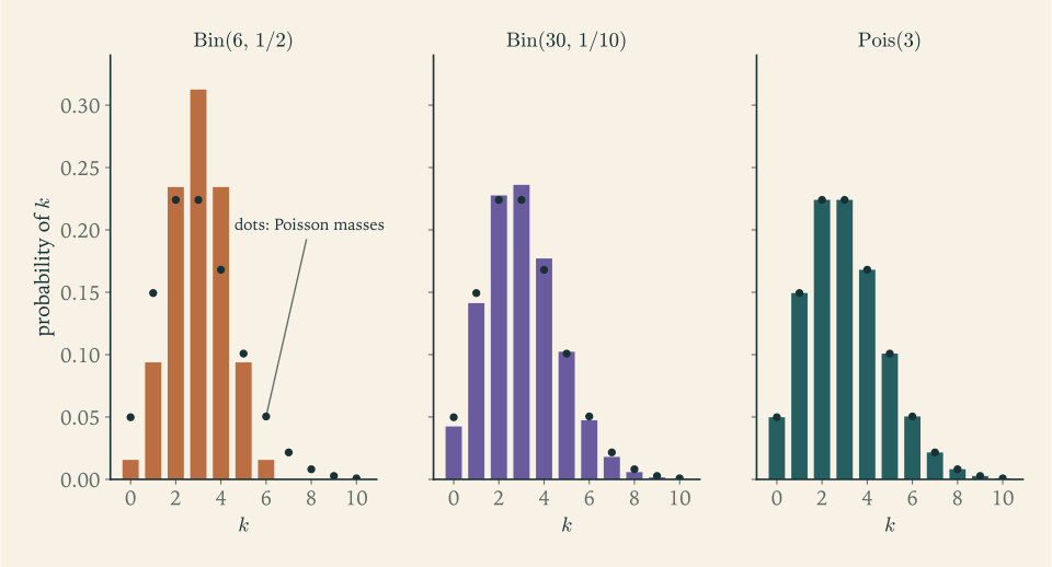
Figure 3.1 shows the convergence in Theorem 3.12 happening. With six trials the distribution is visibly different: it is symmetric and stops at six. With thirty trials each bar is within about \(0.012\) of the Poisson bar. The approximation is good when \(n\) is large and \(p\) is small; it does not require any particular value of \(np\) .
The Poisson distribution is the natural model for a count when events occur singly, at a constant average rate, and independently in disjoint stretches of time or space. Making that statement precise leads to the Poisson process, which is developed in Stochastic Processes (math.stochastic-processes.poisson-arrivals).
3.7 Probability generating functions
A distribution on the nonnegative integers is a sequence of numbers \(p(0),p(1),p(2),\dots\) A productive idea, used throughout mathematics, is to package a sequence as the coefficients of a power series and then work with the function instead of the sequence.
Definition 3.13 (probability generating function). Let \(X\) take values in \(\{0,1,2,\dots\}\) . Its probability generating function is
defined for all real \(s\) at which the series converges absolutely, which includes every \(s\) with \(\lvert s\rvert\le 1\) .
The series converges for \(\lvert s\rvert\le 1\) because its terms are dominated by the masses, which sum to one. Always \(G_X(1)=1\) and \(G_X(0)=P(X=0)\) .
Theorem 3.14 (what a generating function determines). Let \(X\) take values in \(\{0,1,2,\dots\}\) with generating function \(G\) .
(a) For every \(k\ge 0\) , \(P(X=k)=G^{(k)}(0)/k!\) . Hence two such random variables with the same generating function on an interval around \(0\) have the same distribution.
(b) If the series for \(G\) converges on an interval \(\lvert s\rvert<\rho\) with \(\rho>1\) , then \(E[X]=G'(1)\) and \(E[X(X-1)]=G''(1)\) , so that
Proof. A power series may be differentiated term by term inside its interval of convergence, a standard result of Real Analysis. Differentiating \(k\) times and setting \(s=0\) leaves only the term with index \(k\) , namely \(k!\,p_X(k)\) ; this is (a). For (b), the point \(s=1\) is inside the interval of convergence, and term-by-term differentiation gives \(G'(s)=\sum_k k\,p_X(k)s^{k-1}\) and \(G''(s)=\sum_k k(k-1)p_X(k)s^{k-2}\) . At \(s=1\) these are \(E[X]\) and \(E[X(X-1)]\) by Theorem 3.4. Finally \(E[X^2]=E[X(X-1)]+E[X]\) .
When the series converges only for \(\lvert s\rvert\le 1\) , part (b) remains true if \(G'(1)\) and \(G''(1)\) are read as limits from the left, possibly infinite; we shall not need that refinement.
The generating functions of the standard distributions are closed-form expressions.
Binomial. By the binomial theorem, \(G(s)=\sum_k\binom nk(ps)^kq^{n-k}=(q+ps)^n\) .
Geometric. \(G(s)=\sum_{k\ge 1}q^{k-1}p\,s^k=\dfrac{ps}{1-qs}\) for \(\lvert s\rvert<1/q\) .
Poisson. \(G(s)=e^{-\lambda}\sum_k\dfrac{(\lambda s)^k}{k!}=e^{\lambda(s-1)}\) for all \(s\) .
Example 3.7: Moments of the geometric distribution without summing series
For \(T\sim\mathrm{Geom}(p)\) , differentiate \(G(s)=ps/(1-qs)\) :
At \(s=1\) , where \(1-q=p\) , these give \(G'(1)=1/p\) and \(G''(1)=2q/p^2\) . Hence \(E[T]=1/p\) , confirming the tail-sum computation, and
For the wait for a six, \(p=1/6\) , the mean is \(6\) and the variance is \(30\) , a standard deviation of about \(5.5\) rolls. The wait is highly variable: its standard deviation is nearly as large as its mean.
The same two derivatives of \((q+ps)^n\) give \(np\) and \(n(n-1)p^2\) , recovering the binomial variance \(npq\) ; and those of \(e^{\lambda(s-1)}\) give \(\lambda\) and \(\lambda^2\) .
Generating functions also turn limits of distributions into limits of functions. If \(np_n=\lambda\) , the binomial generating function is \(\bigl(1+\lambda(s-1)/n\bigr)^n\) , which converges to \(e^{\lambda(s-1)}\) for every \(s\) . The limit is the Poisson generating function, which matches Theorem 3.12; and it is a general fact, not proved here, that when the limit is the generating function of a probability distribution, convergence of generating functions on \([0,1]\) is equivalent to convergence of every mass.
One further property makes generating functions indispensable, and it must wait for the notion of independent random variables in Chapter 5: the generating function of a sum of independent variables is the product of their generating functions, which explains at a glance why \((q+ps)^n\) is an \(n\) -th power. Chapter 4 introduces a close relative, the moment generating function, which works for random variables that are not integer-valued, and Chapter 8 uses it to prove the central limit theorem.
Exercises
-
Two fair dice are rolled and \(D\) is the absolute difference of the numbers shown. Find the probability mass function of \(D\) , check that it sums to one, and compute \(E[D]\) .
Answer
Counting ordered pairs: \(p_D(0)=\tfrac{6}{36}\) , \(p_D(1)=\tfrac{10}{36}\) , \(p_D(2)=\tfrac{8}{36}\) , \(p_D(3)=\tfrac{6}{36}\) , \(p_D(4)=\tfrac{4}{36}\) , \(p_D(5)=\tfrac{2}{36}\) ; in general \(p_D(d)=2(6-d)/36\) for \(d\ge 1\) . The masses sum to \(36/36\) , and \(E[D]=(10+16+18+16+10)/36=70/36=35/18\approx 1.94\) .
-
Let \(X\) have mass function \(p(k)=\dfrac{c}{k(k+1)}\) for \(k=1,2,3,\dots\) Find the constant \(c\) , show that \(E[X]=\infty\) , and find \(P(X>n)\) for each \(n\ge 1\) .
Solution
Since \(\dfrac{1}{k(k+1)}=\dfrac1k-\dfrac1{k+1}\) , the partial sums telescope:
\[ \sum_{k=1}^{n}\frac{1}{k(k+1)}=1-\frac{1}{n+1}\longrightarrow 1 . \]The masses must sum to one, so \(c=1\) . The same telescoping gives the tail: \(P(X>n)=1-P(X\le n)=\dfrac{1}{n+1}\) .
For the expectation, the values are positive, so the definition gives
\[ E[X]=\sum_{k=1}^{\infty}k\cdot\frac{1}{k(k+1)}=\sum_{k=1}^{\infty}\frac{1}{k+1}, \]which is the harmonic series without its first term and diverges. Hence \(E[X]=\infty\) . The tail-sum formula says the same: \(\sum_{k\ge 1}P(X\ge k)=\sum_{k\ge 1}\tfrac1k=\infty\) . The distribution is perfectly well defined and \(X\) is finite with probability one; its tail simply decays too slowly, like \(1/n\) , for the mean to be finite.
-
Let \(X\) be equally likely to take each of the values \(-2,-1,0,1,2\) . Find the mass function of \(Y=X^2\) and compute \(E[Y]\) twice, once from the mass function of \(Y\) and once from Theorem 3.4.
Answer
\(Y\) takes the values \(0,1,4\) with masses \(\tfrac15,\tfrac25,\tfrac25\) . From this, \(E[Y]=0+\tfrac25+\tfrac85=2\) . From Theorem 3.4, \(E[X^2]=\tfrac15(4+1+0+1+4)=2\) .
-
In the birthday model with \(n\) people, use indicators of the events “nobody is born on day \(d\) ” to find the expected number of distinct birthdays, and evaluate it for \(n=23\) .
Solution
Let \(B_d\) be the event that nobody is born on day \(d\) , for \(d=1,\dots,365\) . Each person independently avoids day \(d\) with probability \(364/365\) , so \(P(B_d)=(364/365)^n\) . The number of days on which nobody is born is \(\sum_d\mathbf 1_{B_d}\) , with expectation \(365\,(364/365)^n\) by linearity. The number of distinct birthdays is \(365\) minus that count, so
\[ E[\text{distinct birthdays}]=365\Bigl(1-\Bigl(\frac{364}{365}\Bigr)^{n}\Bigr). \]For \(n=23\) this is about \(22.32\) . So among \(23\) people the expected number of “lost” birthdays, \(23-22.32=0.68\) , is less than one, even though a shared birthday is more likely than not. The events \(B_d\) are far from independent (their indicators must sum to at least \(365-n\) ), and linearity does not care.
-
A coin with probability \(p\) of heads is tossed \(n\) times. A run is a maximal block of consecutive equal results, so that HHTHTT has four runs. Find the expected number of runs, and evaluate it for ten tosses of a fair coin.
Solution
A new run starts at toss \(1\) , and at toss \(i\ge 2\) exactly when toss \(i\) differs from toss \(i-1\) . So the number of runs is
\[ R=1+\sum_{i=2}^{n}\mathbf 1_{C_i},\qquad C_i=\{\text{tosses } i-1 \text{ and } i \text{ differ}\}. \]By independence of the tosses, \(P(C_i)=p(1-p)+(1-p)p=2p(1-p)\) . Linearity gives
\[ E[R]=1+2(n-1)p(1-p). \]For ten tosses of a fair coin, \(E[R]=1+9\cdot\tfrac12=5.5\) . The events \(C_i\) and \(C_{i+1}\) share a toss, but the mean is unaffected by any dependence between them. The expected number of runs is largest for a fair coin and falls to \(1\) as \(p\) approaches \(0\) or \(1\) , when the sequence is almost surely constant.
-
Let \(X\) have finite variance and mean \(\mu\) . Prove that \(E[(X-c)^2]=\operatorname{Var}(X)+(\mu-c)^2\) for every real \(c\) , and conclude that the mean is the unique constant minimizing the expected squared distance to \(X\) .
Solution
Write \(X-c=(X-\mu)+(\mu-c)\) and expand the square:
\[ (X-c)^2=(X-\mu)^2+2(\mu-c)(X-\mu)+(\mu-c)^2 . \]Take expectations using linearity. The middle term has expectation \(2(\mu-c)\,E[X-\mu]=0\) , because \(E[X-\mu]=\mu-\mu=0\) , and the last term is a constant. Therefore
\[ E[(X-c)^2]=\operatorname{Var}(X)+(\mu-c)^2 . \]The first term does not depend on \(c\) and the second is nonnegative, vanishing only when \(c=\mu\) . So \(c=\mu\) is the unique minimizer, and the minimum value is the variance. This is the probabilistic form of the parallel-axis theorem in mechanics, and it is the reason the variance is defined with deviations from the mean and not from some other centre.
-
A student reasons: “The expected number of rolls of a fair die needed to get a six is \(6\) , so there is a fifty percent chance of getting a six within \(6\) rolls.” Compute the probability of a six within \(6\) rolls, find the smallest number of rolls for which that probability is at least one half, and explain what the student confused.
Solution
The number of rolls \(T\) needed for the first six is geometric with \(p=1/6\) , so \(P(T\le n)=1-(5/6)^n\) . For \(n=6\) this is \(1-(5/6)^6\approx 0.665\) , not one half. Since \(1-(5/6)^3\approx 0.421\) and \(1-(5/6)^4\approx 0.518\) , the smallest number of rolls giving at least an even chance is \(4\) .
The student confused the mean with the median. The mean, \(6\) , is the balance point of the distribution. The median is the value that splits the probability in half, and here it is \(4\) . The geometric distribution is strongly skewed to the right: occasional very long waits pull the mean well above the median. An expectation by itself says nothing about the probability of being below it; for that one needs the distribution, or at least an inequality of the kind developed in Chapter 7.
-
For \(X\sim\mathrm{Bin}(10,0.3)\) compute \(P(X=3)\) and \(P(X\ge 5)\) to four decimal places, and determine the most likely value of \(X\) by examining the ratio \(P(X=k+1)/P(X=k)\) .
Answer
\(P(X=3)=\binom{10}{3}0.3^3\,0.7^7\approx 0.2668\) and \(P(X\ge 5)\approx 0.1503\) . The ratio \(P(X=k+1)/P(X=k)=\dfrac{(10-k)\,0.3}{(k+1)\,0.7}\) exceeds \(1\) exactly when \(k<2.3\) , so the masses increase up to \(k=3\) and decrease afterwards; the most likely value is \(3\) .
-
Let \(T\) take values in \(\{1,2,3,\dots\}\) with \(P(T>1)=q\) where \(0<q<1\) , and suppose \(P(T>m+n)=P(T>m)\,P(T>n)\) for all integers \(m,n\ge 0\) , which is the lack-of-memory property written without a conditional probability. Prove that \(T\) is geometric.
Hint
Put \(t(n)=P(T>n)\) . The hypothesis says \(t(m+n)=t(m)\,t(n)\) . Deduce \(t(n)=t(1)^n=q^n\) by induction, and then compute \(P(T=k)=t(k-1)-t(k)\) .
-
Five cards are dealt from a standard deck and \(X\) is the number of hearts. Write the mass function of \(X\) , compute \(P(X=2)\) , and find \(E[X]\) by indicators.
Answer
\(P(X=k)=\binom{13}{k}\binom{39}{5-k}/\binom{52}{5}\) for \(k=0,\dots,5\) . \(P(X=2)=\dfrac{78\cdot 9139}{2{,}598{,}960}\approx 0.2743\) . Each of the five cards is a heart with probability \(\tfrac14\) , so \(E[X]=\tfrac54\) .
-
Independent trials succeed with probability \(0.4\) . Find the probability that the third success occurs on the seventh trial, and the expected number of trials needed for three successes.
Answer
\(\binom{6}{2}0.4^3\,0.6^4=15\cdot 0.064\cdot 0.1296\approx 0.1244\) . The expected number of trials is \(3/0.4=7.5\) .
-
Misprints on a page follow a Poisson distribution with mean \(0.5\) , independently from page to page. Find the probability that a page has no misprints, the probability that it has at least two, and the probability that at least one page in a ten-page chapter has at least two.
Solution
Let \(X\) be the number of misprints on a page, \(X\sim\mathrm{Pois}(0.5)\) . Then
\[ P(X=0)=e^{-0.5}\approx 0.6065,\qquad P(X\ge 2)=1-e^{-0.5}(1+0.5)\approx 0.0902 . \]For the chapter, the ten pages are independent, and each has at least two misprints with probability \(r\approx 0.0902\) . The probability that at least one page does is
\[ 1-(1-r)^{10}\approx 1-0.9098^{10}\approx 0.611 . \]Although a page with two or more misprints is uncommon, there are ten chances, and the complement rule for independent trials from Chapter 2 gives better than even odds that it happens somewhere. The union bound would give \(10r\approx 0.90\) , which is valid but loose here.
-
For \(X\sim\mathrm{Pois}(\lambda)\) , show that \(P(X=k+1)/P(X=k)=\lambda/(k+1)\) and deduce the most likely value or values of \(X\) . Then show that \(P(X\text{ is even})=\tfrac12\bigl(1+e^{-2\lambda}\bigr)\) by adding the series for \(e^{\lambda}\) and \(e^{-\lambda}\) .
Solution
The ratio of consecutive masses is
\[ \frac{P(X=k+1)}{P(X=k)}=\frac{\lambda^{k+1}/(k+1)!}{\lambda^k/k!}=\frac{\lambda}{k+1}. \]The masses increase while \(k+1<\lambda\) and decrease once \(k+1>\lambda\) . If \(\lambda\) is not an integer, the unique most likely value is the integer part of \(\lambda\) . If \(\lambda\) is an integer, the ratio equals \(1\) at \(k=\lambda-1\) , so \(\lambda-1\) and \(\lambda\) are both most likely; for \(\lambda<1\) the mode is \(0\) .
For the parity, add the two exponential series: in \(e^{\lambda}+e^{-\lambda}=\sum_k\bigl(1+(-1)^k\bigr)\lambda^k/k!\) the odd terms cancel and the even terms double, so \(\sum_{k\text{ even}}\lambda^k/k!=\tfrac12(e^{\lambda}+e^{-\lambda})\) . Multiplying by \(e^{-\lambda}\) ,
\[ P(X\text{ is even})=\tfrac12\bigl(1+e^{-2\lambda}\bigr). \]This exceeds one half for every \(\lambda\) , because \(0\) is even, and tends to one half as \(\lambda\) grows. The same result is \(\tfrac12\bigl(G(1)+G(-1)\bigr)\) with \(G(s)=e^{\lambda(s-1)}\) , a general identity for generating functions.
-
Each of \(500\) people is born on the first of January with probability \(1/365\) , independently. Compute the probability that exactly two of them are, once from the binomial distribution and once from its Poisson approximation, and compare.
Answer
Binomial: \(\binom{500}{2}(1/365)^2(364/365)^{498}\approx 0.2388\) . Poisson with \(\lambda=500/365\approx 1.370\) : \(e^{-\lambda}\lambda^2/2\approx 0.2385\) . They differ by about \(0.0004\) .
-
Find the probability generating function of the result of one roll of a fair die, and use Theorem 3.14 to compute its mean and variance.
Answer
\(G(s)=\tfrac16(s+s^2+\dots+s^6)\) . \(G'(1)=\tfrac{21}{6}=\tfrac72\) and \(G''(1)=\tfrac16(2+6+12+20+30)=\tfrac{35}{3}\) , so the mean is \(\tfrac72\) and the variance is \(\tfrac{35}{3}+\tfrac72-\tfrac{49}{4}=\tfrac{35}{12}\) .
-
A random variable \(X\) on the nonnegative integers has generating function \(G(s)=\dfrac{s^2}{(2-s)^2}\) . Expand \(G\) as a power series to find the mass function of \(X\) , compute \(E[X]\) and \(\operatorname{Var}(X)\) from derivatives of \(G\) , and identify the distribution from the table in Section 3.5.
Solution
Write \(G(s)=\dfrac{s^2}{4}\Bigl(1-\dfrac s2\Bigr)^{-2}\) . Differentiating the geometric series \(\sum_m x^m=(1-x)^{-1}\) gives \((1-x)^{-2}=\sum_{m\ge 0}(m+1)x^m\) , so with \(x=s/2\) ,
\[ G(s)=\sum_{m=0}^{\infty}\frac{m+1}{2^{m+2}}\,s^{m+2}. \]Reading off the coefficient of \(s^k\) with \(k=m+2\) : \(P(X=k)=\dfrac{k-1}{2^k}\) for \(k\ge 2\) . The first few masses are \(\tfrac14,\tfrac14,\tfrac{3}{16},\tfrac18\) .
For the moments, \(G'(s)=\dfrac{4s}{(2-s)^3}\) and \(G''(s)=\dfrac{8(1+s)}{(2-s)^4}\) , so \(G'(1)=4\) and \(G''(1)=16\) . Therefore \(E[X]=4\) and \(\operatorname{Var}(X)=16+4-16=4\) .
The mass function \((k-1)2^{-k}=\binom{k-1}{1}\bigl(\tfrac12\bigr)^2\bigl(\tfrac12\bigr)^{k-2}\) is negative binomial with \(r=2\) and \(p=\tfrac12\) : the number of tosses of a fair coin needed for the second head. The table confirms the mean \(r/p=4\) and variance \(rq/p^2=4\) . Notice also that \(G(s)=\bigl(\tfrac{s}{2-s}\bigr)^2\) is the square of the generating function of \(\mathrm{Geom}(\tfrac12)\) .
-
Use the tail-sum formula to find the expected value of the smaller of the two numbers when two fair dice are rolled, and check that the expected smaller and expected larger numbers add up to the expected sum.
Answer
For the smaller number \(L\) , \(P(L\ge k)=\bigl((7-k)/6\bigr)^2\) , so \(E[L]=(36+25+16+9+4+1)/36=91/36\approx 2.53\) . Since the smaller and larger numbers add up to the sum of the two dice, \(E[L]+E[M]=\tfrac{91}{36}+\tfrac{161}{36}=7\) .
-
A fair die is rolled ten times. Find the expected number of faces that have not appeared, and compare with the probability, from Chapter 1 methods, that all six faces have appeared.
Answer
Each face fails to appear with probability \((5/6)^{10}\) , so the expected number of missing faces is \(6(5/6)^{10}\approx 0.969\) . By inclusion–exclusion the probability that all six have appeared is \(\sum_{k=0}^{6}(-1)^k\binom6k\bigl(\tfrac{6-k}{6}\bigr)^{10}\approx 0.272\) . An expected count near one is compatible with a probability of only about \(0.73\) that at least one face is missing.
-
Three balls are thrown independently into three boxes as in Exercise 19 of Chapter 1Chapter 1. Use indicators to find the mean and the variance of the number of empty boxes, and verify both against the distribution found in that exercise.
Solution
Let \(E_i\) be the event that box \(i\) is empty, \(i=1,2,3\) , and \(X=\mathbf 1_{E_1}+\mathbf 1_{E_2}+\mathbf 1_{E_3}\) the number of empty boxes. Each ball avoids box \(i\) with probability \(\tfrac23\) , independently, so \(P(E_i)=(2/3)^3=\tfrac{8}{27}\) and
\[ E[X]=3\cdot\frac{8}{27}=\frac89 . \]For the variance, square the sum as in Example 3.4. Two given boxes are both empty exactly when all three balls land in the third, so \(P(E_i\cap E_j)=(1/3)^3=\tfrac1{27}\) for \(i\ne j\) , and there are six ordered pairs:
\[ E[X^2]=\frac{24}{27}+6\cdot\frac{1}{27}=\frac{30}{27}=\frac{10}{9},\qquad \operatorname{Var}(X)=\frac{10}{9}-\frac{64}{81}=\frac{26}{81}. \]Verification from the distribution of Exercise 19 of Chapter 1Chapter 1, namely \(P(X=0)=\tfrac{6}{27}\) , \(P(X=1)=\tfrac{18}{27}\) , \(P(X=2)=\tfrac{3}{27}\) : the mean is \((18+6)/27=\tfrac89\) and the second moment is \((18+12)/27=\tfrac{10}{9}\) , in agreement.
-
In the St Petersburg game of Example 3.2, suppose the bank can pay at most \(2^{20}\) units, so that the payoff is the smaller of \(2^k\) and \(2^{20}\) when the first head appears on toss \(k\) . Find the expected payoff, and comment on how it compares with the uncapped game.
Solution
The first head appears on toss \(k\) with probability \(2^{-k}\) . For \(k\le 20\) the payoff is \(2^k\) , contributing \(2^k\cdot 2^{-k}=1\) to the expectation for each such \(k\) . For \(k>20\) the payoff is capped at \(2^{20}\) , and the total probability of those outcomes is \(P(k>20)=2^{-20}\) , contributing \(2^{20}\cdot 2^{-20}=1\) in all. Hence
\[ E[\text{capped payoff}]=20+1=21 . \]The uncapped game has infinite expectation, but all of that infinity comes from payoffs larger than about a million units, which occur with probability less than one in a million. Against any real bank the game is worth a modest amount: each doubling of the bank’s wealth adds one unit to the fair price. The paradox of the St Petersburg game is produced by taking an unbounded payoff seriously.