Break a stick of unit length at a uniformly random point, keep the left piece, break that piece at a uniformly random point, and again keep the left piece. What is the expected length of what remains?

There is an honest way and a fast way. The honest way is to find the density of the final length, which Example 5.4 showed to be \(-\ln y\) on \((0,1)\) , and integrate. The fast way is to say: whatever the length \(X\) of the first piece, the second break leaves on average half of it; so the answer is the average of \(X/2\) , namely \(\tfrac14\) . The fast way is correct, and the sentence “the average of the conditional average is the average” is a theorem. It is one of the most useful in probability, because it lets a problem be solved in stages, each stage conditional on the one before.

To state it, the conditional average has to be treated as an object in its own right. For each possible value \(x\) of \(X\) there is a conditional mean of \(Y\) ; assembling these gives a function of \(x\) ; and evaluating that function at the random value of \(X\) gives a new random variable. This chapter is about that random variable: how to compute with it, how it decomposes variance, and in what sense it is the best prediction of \(Y\) that can be made from \(X\) .

6.1 Averages given an event, and first-step arguments

This is the expectation of \(Y\) under the conditional probability measure \(P(\cdot\mid A)\) of Proposition 2.2: for discrete \(Y\) it equals \(\sum_y y\,P(Y=y\mid A)\) . It averages \(Y\) over the outcomes in \(A\) only.

The statement holds for countably infinite partitions as well. It is the law of total probability with an expectation in place of a probability, and taking \(Y=\mathbf 1_A\) recovers Theorem 2.5. Its most characteristic use is to condition on the first step of a process that then restarts.

6.2 The conditional mean as a function and as a random variable

In the discrete case this is Definition 6.1 with \(A=\{X=x\}\) . In the continuous case that event has probability zero, and the definition rests on the conditional density of Definition 5.3. More generally, \(E[g(X,Y)\mid X=x]\) is computed by putting \(g(x,y)\) in place of \(y\) under the sum or integral: inside a conditional expectation given \(X=x\) , the variable \(X\) may be replaced by the number \(x\) , while \(Y\) is averaged with its conditional distribution.

6.3 Conditional variance and the decomposition of variance

It is the variance of the conditional distribution of \(Y\) , evaluated at the random value of \(X\) , and like the conditional mean it is a random variable. The two forms agree by expanding the square and using rules (a) and (b).

The two terms have distinct meanings. Think of \(X\) as sorting the population into groups. The first term is the average variance within groups. The second is the variance between groups, that is, of the group means. Total variability is the sum of the two, and neither alone suffices.

6.4 The best predictor

Suppose \(X\) will be observed and \(Y\) must then be predicted by some function \(g(X)\) . If the cost of an error is its square, which function is best?

The vanishing cross term says that the prediction error \(Y-E[Y\mid X]\) is uncorrelated with every function of \(X\) : nothing in \(X\) can be used to improve the prediction further. This is the same geometry as the orthogonal projection of a vector onto a subspace in linear algebra, where the error of the best approximation is perpendicular to the subspace (math.linear-algebra.projection-as-best-approximation). Here the “subspace” consists of the functions of \(X\) and “perpendicular” means uncorrelated. With no information at all, the best constant predictor is \(E[Y]\) , with error \(\operatorname{Var}(Y)\) ; the law of total variance then says that observing \(X\) reduces the mean squared error by exactly \(\operatorname{Var}(E[Y\mid X])\) .

Often the regression function is unknown or awkward, and one settles for the best straight line.

Three predictors are now ranked: the constant \(\mu_Y\) , the best line, and the regression function, with mean squared errors

The correlation coefficient measures exactly how much a straight line helps, and says nothing about how much more a curve could help. When the regression function happens to be linear, the last two coincide. That is the case for the standard bivariate normal pair of Section 5.7, where \(E[Y\mid X]=\rho X\) and the conditional variance is \(1-\rho^2\) . Since \(\lvert\rho\rvert<1\) , the predicted value \(\rho x\) is closer to the mean than \(x\) is. An extreme value of \(X\) is expected to be accompanied by a less extreme value of \(Y\) , a phenomenon known as regression to the mean, which is a consequence of imperfect correlation and needs no causal explanation.

Example 6.7: A strong relationship that no line can see

Let \(X\sim\mathrm{Unif}(-1,1)\) and \(Y=X^2+\varepsilon\) , where \(\varepsilon\) is independent of \(X\) with mean \(0\) and standard deviation \(0.1\) . By rules (a), (b), and (c) of Theorem 6.6,

\[ E[Y\mid X]=X^2+E[\varepsilon]=X^2,\qquad \operatorname{Var}(Y\mid X)=\operatorname{Var}(\varepsilon)=0.01 . \]

The best predictor is the parabola \(x^2\) , with mean squared error \(0.01\) .

For the best line we need the covariance: \(\operatorname{Cov}(X,Y)=E[X^3]+E[X\varepsilon]-E[X]E[Y]=0\) , all three terms vanishing by symmetry and independence. So \(\rho=0\) , the best line is the horizontal line at \(E[Y]=E[X^2]=\tfrac13\) , and its mean squared error is the whole variance of \(Y\) :

\[ \operatorname{Var}(Y)=\operatorname{Var}(X^2)+0.01=\Bigl(\tfrac15-\tfrac19\Bigr)+0.01=\tfrac{4}{45}+0.01\approx 0.099 . \]

The parabola’s error is about a tenth of the line’s.

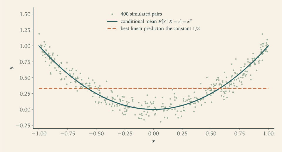
Figure 6.1 makes the three-way ranking visible. The vertical scatter about the curve is the within-group variability \(E[\operatorname{Var}(Y\mid X)]\) , small here. The rise and fall of the curve itself is the between-group variability \(\operatorname{Var}(E[Y\mid X])=\tfrac{4}{45}\) , large here, and entirely invisible to covariance.

6.5 Conditioning on a continuous quantity that is never observed

The law of total probability and Bayes’ rule extend to the case in which the hypothesis is the value of a continuous random variable and the evidence is discrete. If \(\Theta\) has density \(\pi\) and, given \(\Theta=\theta\) , the discrete variable \(X\) has mass function \(p(x\mid\theta)\) , then by the tower property applied to the indicator of \(\{X=x\}\) ,

and the conditional density of \(\Theta\) given \(X=x\) is

These are Theorems 2.5 and 2.6 with an integral over hypotheses.

Exercises

1. For the joint mass function of Exercise 1 of Chapter 5Chapter 5, find \(E[Y\mid X=0]\) and \(E[Y\mid X=1]\) , describe \(E[Y\mid X]\) as a random variable by listing its values and their probabilities, and verify the tower property.

   Answer

   Given \(X=0\) the conditional masses of \(Y\) are \(\tfrac14,\tfrac12,\tfrac14\) , so \(E[Y\mid X=0]=1\) . Given \(X=1\) they are \(\tfrac12,\tfrac16,\tfrac13\) , so \(E[Y\mid X=1]=\tfrac16+\tfrac23=\tfrac56\) . The random variable \(E[Y\mid X]\) equals \(1\) with probability \(0.4\) and \(\tfrac56\) with probability \(0.6\) ; its mean is \(0.4+0.5=0.9=E[Y]\) .

2. A fair die is rolled, and then a fair coin is tossed as many times as the number shown. Find the mean and the variance of the number of heads.

   Solution

   Let \(N\) be the number shown by the die and \(Y\) the number of heads. Given \(N=n\) , \(Y\sim\mathrm{Bin}(n,\tfrac12)\) , so

   \[ E[Y\mid N]=\tfrac12N,\qquad \operatorname{Var}(Y\mid N)=\tfrac14N . \]

   A fair die has \(E[N]=\tfrac72\) and \(\operatorname{Var}(N)=\tfrac{35}{12}\) . By the tower property \(E[Y]=\tfrac12\cdot\tfrac72=\tfrac74\) . By the law of total variance,

   \[ \operatorname{Var}(Y)=E\bigl[\tfrac14N\bigr]+\operatorname{Var}\bigl(\tfrac12N\bigr)=\tfrac78+\tfrac14\cdot\tfrac{35}{12}=\tfrac{42}{48}+\tfrac{35}{48}=\tfrac{77}{48}\approx 1.60 . \]

   The first term is the coin-tossing variability for a given number of coins, and the second is the contribution of not knowing how many coins there are. This is Proposition 6.9 with Bernoulli terms: \(\sigma^2E[N]+\mu^2\operatorname{Var}(N)\) with \(\mu=\tfrac12\) and \(\sigma^2=\tfrac14\) .

3. For the uniform distribution on the triangle \(0<x<y<1\) of Example 5.3, find \(E[Y\mid X]\) and \(\operatorname{Var}(Y\mid X)\) , and verify both the tower property and the law of total variance against the marginal density \(f_Y(y)=2y\) .

   Solution

   Given \(X=x\) , \(Y\) is uniform on \((x,1)\) , by Example 5.4. So

   \[ E[Y\mid X]=\frac{1+X}{2},\qquad \operatorname{Var}(Y\mid X)=\frac{(1-X)^2}{12}. \]

   The marginal density of \(X\) is \(2(1-x)\) , with \(E[X]=\tfrac13\) and \(\operatorname{Var}(X)=\tfrac1{18}\) . Tower property: \(E[Y]=\tfrac12\bigl(1+\tfrac13\bigr)=\tfrac23\) , which matches \(\int_0^1y\cdot 2y\,dy=\tfrac23\) .

   For the variance decomposition,

   \[ E\bigl[\operatorname{Var}(Y\mid X)\bigr]=\frac1{12}\int_0^1(1-x)^2\cdot 2(1-x)\,dx=\frac{1}{12}\cdot\frac12=\frac1{24},\qquad \operatorname{Var}\bigl(E[Y\mid X]\bigr)=\frac14\operatorname{Var}(X)=\frac{1}{72}. \]

   Their sum is \(\tfrac{3}{72}+\tfrac1{72}=\tfrac1{18}\) . Directly from \(f_Y(y)=2y\) : \(E[Y^2]=\int_0^12y^3\,dy=\tfrac12\) and \(\operatorname{Var}(Y)=\tfrac12-\tfrac49=\tfrac1{18}\) . The two agree. Three quarters of the variance of the larger point is within-group, that is, remains after the smaller point is known.

4. A fair die is rolled repeatedly. Use a first-step argument with two states to find the expected number of rolls until two consecutive sixes appear.

   Solution

   Let \(a\) be the expected number of rolls from the start and \(b\) the expected number of further rolls when the last roll was a six. From the start, one roll is used, after which we are in the “six” state with probability \(\tfrac16\) and back at the start otherwise. From the “six” state, one roll is used; a six finishes, anything else returns us to the start. Hence

   \[ a=1+\tfrac16b+\tfrac56a,\qquad b=1+\tfrac56a . \]

   The first equation gives \(a=6+b\) . Substituting into the second, \(b=1+\tfrac56(6+b)=6+\tfrac56b\) , so \(b=36\) and

   \[ a=42 . \]

   The answer is \(6+36\) : six rolls on average to get one six, and then, because a failure at the second stage throws away the first six, the structure \(a=\tfrac1p+\tfrac1{p^2}\) with \(p=\tfrac16\) . For a fair coin the same formula gives \(2+4=6\) , the value found in Example 6.1.

5. A miner is in a chamber with three doors and chooses one at random each time, with no memory of earlier choices. The first door leads out after \(3\) hours; the second returns him to the chamber after \(5\) hours; the third returns him after \(7\) hours. Find the expected time until he gets out, and by conditioning \(T^2\) on the first choice find the variance of that time.

   Answer

   With \(m=E[T]\) : \(m=\tfrac13\cdot 3+\tfrac13(5+m)+\tfrac13(7+m)\) , so \(m=15\) hours. With \(s=E[T^2]\) : \(s=\tfrac13\bigl(9+E[(5+T)^2]+E[(7+T)^2]\bigr)=\tfrac13\bigl(9+25+150+s+49+210+s\bigr)\) , so \(s=443\) and \(\operatorname{Var}(T)=443-225=218\) , a standard deviation of about \(14.8\) hours.

6. Prove that \(E[Y\mid X]=E[Y]\) whenever \(X\) and \(Y\) are independent, and show by the example \(Y\) uniform on \(\{-1,0,1\}\) , \(X=Y^2\) that the converse is false.

   Solution

   If \(X\) and \(Y\) are independent, the conditional distribution of \(Y\) given \(X=x\) is the marginal distribution of \(Y\) : in the discrete case \(p_{Y\mid X}(y\mid x)=p_X(x)p_Y(y)/p_X(x)=p_Y(y)\) , and likewise for densities, by Proposition 5.5. So \(E[Y\mid X=x]=\sum_yy\,p_Y(y)=E[Y]\) for every \(x\) , and \(E[Y\mid X]\) is the constant \(E[Y]\) .

   For the converse, let \(Y\) be uniform on \(\{-1,0,1\}\) and \(X=Y^2\) . Given \(X=1\) , \(Y\) is \(-1\) or \(1\) with probability \(\tfrac12\) each, so \(E[Y\mid X=1]=0\) . Given \(X=0\) , \(Y=0\) , so \(E[Y\mid X=0]=0\) . Thus \(E[Y\mid X]=0=E[Y]\) identically. But \(X\) and \(Y\) are dependent: \(P(Y=0\mid X=0)=1\) while \(P(Y=0)=\tfrac13\) .

   So there are three conditions of decreasing strength: independence; a constant regression function, sometimes called mean independence; and zero covariance, which follows from the second by Exercise 6.10. Neither implication reverses.

7. Half of a factory’s parts come from machine A, whose parts have lengths that are normal with mean \(10\) and variance \(1\) , and half from machine B, with mean \(14\) and variance \(1\) . A student says the length of a randomly chosen part has variance \(1\) , “since both machines have variance \(1\) ”. Find the correct variance, name the term the student omitted, and say whether the length is normally distributed.

   Solution

   Let \(M\) record the machine and \(L\) the length. Then \(E[L\mid M]\) is \(10\) or \(14\) with probability \(\tfrac12\) each, and \(\operatorname{Var}(L\mid M)=1\) in both cases. The law of total variance gives

   \[ \operatorname{Var}(L)=E[\operatorname{Var}(L\mid M)]+\operatorname{Var}(E[L\mid M])=1+4=5, \]

   since a variable equally likely to be \(10\) or \(14\) has mean \(12\) and variance \(2^2=4\) . The student computed only the within-group term and omitted the between-group term, the variance of the machine means, which here is four times larger.

   The length is not normally distributed. Its density is the equal mixture \(\tfrac12\varphi(x-10)+\tfrac12\varphi(x-14)\) , which has two peaks, near \(10\) and near \(14\) , and a dip between them at \(12\) . A mixture of normal distributions should not be confused with a sum of normal variables: the sum of independent lengths from A and B would be \(N(24,2)\) , by Corollary 5.14.

8. The number of claims an insurer receives in a month is Poisson with mean \(3\) , and claim sizes are independent and uniform on \((0,2)\) , in thousands. Find the mean and the variance of the total claimed.

   Answer

   Claim sizes have \(\mu=1\) and \(E[X^2]=\int_0^2\tfrac12x^2\,dx=\tfrac43\) . By Proposition 6.9 with a Poisson count, \(E[S]=3\cdot 1=3\) and \(\operatorname{Var}(S)=3\cdot\tfrac43=4\) , in thousands and thousands squared.

9. Let \(N\sim\mathrm{Pois}(\lambda)\) be independent of the independent and identically distributed variables \(X_i\) , which have moment generating function \(M_X\) . Show that \(S=X_1+\dots+X_N\) has \(M_S(t)=\exp\bigl(\lambda(M_X(t)-1)\bigr)\) , and recover \(E[S]\) and \(\operatorname{Var}(S)\) by differentiating.

   Hint

   Use Proposition 6.9 with \(G_N(s)=e^{\lambda(s-1)}\) . Then \(M_S'(t)=\lambda M_X'(t)M_S(t)\) and \(M_S''(t)=\bigl(\lambda M_X''(t)+\lambda^2M_X'(t)^2\bigr)M_S(t)\) ; evaluate at \(t=0\) to get \(E[S]=\lambda\mu\) and \(E[S^2]=\lambda E[X^2]+\lambda^2\mu^2\) .

10. Prove that \(\operatorname{Cov}(X,Y)=\operatorname{Cov}\bigl(X,E[Y\mid X]\bigr)\) for random variables with finite variances, and deduce that if the regression function of \(Y\) on \(X\) is constant then \(X\) and \(Y\) are uncorrelated.

    Solution

    Let \(h(X)=E[Y\mid X]\) . By the weighted tower property, rule (d) of Theorem 6.6 with \(g(x)=x\) ,

    \[ E[XY]=E[X\,h(X)], \]

    and by the tower property \(E[Y]=E[h(X)]\) . Therefore

    \[ \operatorname{Cov}(X,Y)=E[XY]-E[X]E[Y]=E[X\,h(X)]-E[X]\,E[h(X)]=\operatorname{Cov}\bigl(X,h(X)\bigr). \]

    Finite variances guarantee that all these expectations exist; \(h(X)\) has finite variance because \(\operatorname{Var}(h(X))\le\operatorname{Var}(Y)\) by the law of total variance.

    If the regression function is constant, \(h(X)=c\) , then \(\operatorname{Cov}(X,c)=0\) by Proposition 5.8(a), so \(\operatorname{Cov}(X,Y)=0\) . In words, the covariance between \(X\) and \(Y\) sees only the part of \(Y\) that is predictable from \(X\) ; the unpredictable remainder \(Y-h(X)\) is uncorrelated with \(X\) .

11. For the density \(x+y\) on the unit square, compute the mean squared errors of three predictors of \(Y\) : the constant \(E[Y]\) , the best linear predictor of Proposition 6.11, and the regression function of Example 6.2. Comment on how much is gained at each step.

    Solution

    From Example 5.6, \(\operatorname{Var}(Y)=\tfrac{11}{144}\) and \(\rho=-\tfrac1{11}\) .

    Constant predictor. The mean squared error of \(E[Y]=\tfrac7{12}\) is \(\operatorname{Var}(Y)=\tfrac{11}{144}\approx 0.07639\) .

    Best line. By Proposition 6.11 the error is \(\sigma_Y^2(1-\rho^2)=\tfrac{11}{144}\cdot\tfrac{120}{121}=\tfrac{5}{66}\approx 0.07576\) . The line is \(\tfrac7{12}-\tfrac1{11}\bigl(x-\tfrac7{12}\bigr)\) .

    Regression function. By Theorem 6.10 the error is \(E[Y^2]-E[h(X)^2]\) with \(h(x)=\dfrac{3x+2}{3(2x+1)}\) and \(f_X(x)=\tfrac12(2x+1)\) :

    \[ E[h(X)^2]=\frac1{18}\int_0^1\frac{(3x+2)^2}{2x+1}\,dx=\frac{1}{18}\Bigl(6+\frac{\ln 3}{8}\Bigr), \]

    using the division \(\dfrac{(3x+2)^2}{2x+1}=\tfrac92x+\tfrac{15}{4}+\dfrac{1/4}{2x+1}\) . With \(E[Y^2]=\tfrac5{12}\) the error is \(\tfrac1{12}-\tfrac{\ln 3}{144}\approx 0.07570\) .

    The three errors are \(0.07639\) , \(0.07576\) , and \(0.07570\) . Knowing \(X\) reduces the mean squared error by less than one percent, and nearly all of that small gain is already captured by the straight line. The dependence between the coordinates is genuine and almost useless for prediction.

12. Standardized heights of fathers and sons form a standard bivariate normal pair with correlation \(0.5\) . For a father two standard deviations above the mean, find the expected standardized height of the son and the probability that the son is also at least two standard deviations above the mean, and compare with the same probability for a son chosen with no information about the father.

    Answer

    Given \(X=2\) , \(Y\sim N(1,\,0.75)\) . So the expected standardized height is \(1\) , and \(P(Y>2\mid X=2)=1-\Phi\bigl(1/\sqrt{0.75}\bigr)=1-\Phi(1.155)\approx 0.124\) , against \(1-\Phi(2)\approx 0.023\) unconditionally. The son of a very tall father is much more likely than average to be very tall, and is still expected to be less extreme than his father.

13. In the model of Example 6.8, a coin is tossed three times and shows three heads. Find the conditional density of \(\Theta\) , the conditional probability that \(\Theta>\tfrac12\) , and the conditional probability that a fourth toss shows a head.

    Solution

    With \(n=3\) and \(k=3\) , Example 6.8 gives the conditional density

    \[ \pi(\theta\mid 3)=\frac{4!}{3!\,0!}\,\theta^3=4\theta^3,\qquad 0<\theta<1 . \]

    It can be checked directly: the likelihood of three heads is \(\theta^3\) , the prior density is \(1\) , and \(\int_0^1\theta^3\,d\theta=\tfrac14\) is the marginal probability of three heads, in agreement with \(1/(n+1)\) . Then

    \[ P\bigl(\Theta>\tfrac12\mid X=3\bigr)=\int_{1/2}^{1}4\theta^3\,d\theta=1-\tfrac1{16}=\tfrac{15}{16}, \]

    and the conditional probability that the fourth toss is a head is the conditional mean of \(\Theta\) ,

    \[ \int_0^1\theta\cdot 4\theta^3\,d\theta=\tfrac45, \]

    which is \((k+1)/(n+2)\) . Three heads in a row move the probability that the coin favours heads from \(\tfrac12\) to \(\tfrac{15}{16}\) , yet the probability of a further head is only \(0.8\) , not \(1\) : the conditional density still gives weight to moderate values of \(\theta\) .

14. A rate \(\Lambda\) is exponential with mean \(1\) , and given \(\Lambda=\lambda\) a lifetime \(T\) is exponential with rate \(\lambda\) . Find \(P(T>t)\) , the density of \(T\) , and \(E[T]\) .

    Solution

    Given \(\Lambda=\lambda\) , \(P(T>t\mid\Lambda=\lambda)=e^{-\lambda t}\) . By the tower property applied to the indicator of \(\{T>t\}\) , with the density \(e^{-\lambda}\) of \(\Lambda\) ,

    \[ P(T>t)=E\bigl[e^{-\Lambda t}\bigr]=\int_0^{\infty}e^{-\lambda t}e^{-\lambda}\,d\lambda=\frac{1}{1+t},\qquad t\ge 0 . \]

    This is the moment generating function of \(\Lambda\) evaluated at \(-t\) . Differentiating, the density of \(T\) is \(f_T(t)=\dfrac{1}{(1+t)^2}\) for \(t>0\) . For the mean, the tail-integral formula gives

    \[ E[T]=\int_0^{\infty}\frac{dt}{1+t}=\infty . \]

    The tower property gives the same: \(E[T\mid\Lambda]=1/\Lambda\) and \(E[1/\Lambda]=\int_0^{\infty}\lambda^{-1}e^{-\lambda}d\lambda=\infty\) . Each conditional distribution has a finite mean and exponentially thin tails, but mixing over the rate, which can be arbitrarily close to zero, produces a heavy-tailed lifetime with no mean. The mixture is not memoryless: surviving a long time is evidence that the rate is small.

15. Let \(X\sim\mathrm{Pois}(\lambda)\) and, given \(X=n\) , let \(Y\sim\mathrm{Bin}(n,p)\) . Use the tower property to compute the probability generating function of \(Y\) and identify its distribution.

    Solution

    Given \(X=n\) , the generating function of \(Y\) is that of \(\mathrm{Bin}(n,p)\) : \(E[s^Y\mid X=n]=(q+ps)^n\) with \(q=1-p\) . By the tower property,

    \[ G_Y(s)=E\bigl[(q+ps)^X\bigr]=G_X(q+ps)=e^{\lambda(q+ps-1)}=e^{\lambda p(s-1)}, \]

    using \(G_X(u)=e^{\lambda(u-1)}\) and \(q-1=-p\) . This is the generating function of \(\mathrm{Pois}(\lambda p)\) , and by Theorem 3.14(a) a generating function determines the distribution. So \(Y\sim\mathrm{Pois}(\lambda p)\) .

    Interpretation: if a Poisson number of events occurs and each is independently kept with probability \(p\) , the number kept is again Poisson, with the mean reduced by the factor \(p\) . This thinning property is the counterpart of the closure of Poisson variables under independent sums in Corollary 5.14, and Exercise 14 of Chapter 5Chapter 5 showed the reverse direction, from a Poisson total to a binomial share.

16. Let \(X\sim\mathrm{Exp}(1)\) . Find \(E[X\mid X>1]\) and \(E[X\mid X<1]\) , and verify the law of total expectation for the partition into these two events.

    Answer

    By lack of memory \(E[X\mid X>1]=1+1=2\) . \(E[X\mid X<1]=\dfrac{\int_0^1xe^{-x}dx}{1-e^{-1}}=\dfrac{1-2e^{-1}}{1-e^{-1}}\approx 0.418\) . Check: \(2e^{-1}+\bigl(1-2e^{-1}\bigr)=1=E[X]\) .

17. Two fair dice are rolled; \(X\) is the first die and \(M\) the larger of the two. Tabulate \(E[M\mid X=k]\) for \(k=1,\dots,6\) and use the tower property to recover \(E[M]\) from Example 3.2.

    Answer

    Given \(X=k\) , \(M=k\) if the second die shows at most \(k\) and equals the second die otherwise, so \(E[M\mid X=k]=\dfrac{k^2+(k+1)+\dots+6}{6}\) , giving \(\tfrac72,\tfrac{11}{3},4,\tfrac92,\tfrac{31}{6},6\) for \(k=1,\dots,6\) . Their average is \(\tfrac{161}{36}\) .

18. Prove rule (b) of Theorem 6.6 in the discrete case directly from Definition 6.3, and use it together with the tower property to show that \(E\bigl[(Y-E[Y\mid X])\,g(X)\bigr]=0\) .

    Hint

    Given \(X=x\) , \(E[g(X)Y\mid X=x]=\sum_yg(x)\,y\,p_{Y\mid X}(y\mid x)\) , and \(g(x)\) does not depend on \(y\) . For the second part apply the tower property to \((Y-h(X))g(X)\) and take \(g(X)\) out of the inner conditional expectation; what is left inside is \(E[Y\mid X]-h(X)=0\) .

19. Define the correlation ratio \(\eta^2=\operatorname{Var}(E[Y\mid X])/\operatorname{Var}(Y)\) . Use the ranking of predictors in Section 6.4 to prove that \(\rho^2\le\eta^2\le 1\) , and state when each equality holds.

    Hint

    The ranking gives \(\sigma_Y^2(1-\rho^2)\ge E[\operatorname{Var}(Y\mid X)]=\sigma_Y^2-\operatorname{Var}(E[Y\mid X])\) , by the law of total variance; rearrange. Equality \(\rho^2=\eta^2\) holds when the regression function is linear, and \(\eta^2=1\) when \(Y\) is a function of \(X\) with probability one.

20. Let \(X\sim\mathrm{Exp}(1)\) and, given \(X=x\) , let \(Y\sim\mathrm{Pois}(x)\) . Find \(P(Y=k)\) for every \(k\ge 0\) , identify the distribution, and compute \(E[Y]\) and \(\operatorname{Var}(Y)\) both from that distribution and from the tower property and the law of total variance.

    Answer

    \(P(Y=k)=\int_0^{\infty}e^{-x}\dfrac{x^k}{k!}e^{-x}\,dx=\dfrac{1}{k!}\cdot\dfrac{k!}{2^{k+1}}=2^{-(k+1)}\) for \(k\ge 0\) : one less than a \(\mathrm{Geom}(\tfrac12)\) variable. So \(E[Y]=2-1=1\) and \(\operatorname{Var}(Y)=q/p^2=2\) . By conditioning, \(E[Y]=E[X]=1\) and \(\operatorname{Var}(Y)=E[X]+\operatorname{Var}(X)=1+1=2\) .