Set the gradient of \(f(x,y)=x^4+y^4-4xy\) to zero and three points appear: \((0,0)\) , \((1,1)\) , and \((-1,-1)\) . Which of them, if any, minimizes \(f\) ? The gradient cannot say, because it is zero at all three. Something beyond first derivatives must separate a valley floor from a mountain pass, and something beyond local information must decide whether a valley floor is the lowest one.
This chapter treats minimization over all of \(\mathbb R^n\) , or over an open set, where every small move is allowed. It proves the first-order necessary condition, the second-order necessary and sufficient conditions, and the statement that makes convex problems special: for a convex function a vanishing gradient is not merely necessary but sufficient, and globally so. Quadratic functions and least-squares problems are worked out completely, since they are both the simplest instances and the local model of everything else.
3.1 The gradient must vanish
Theorem 3.1 (first-order necessary condition). Let \(f\) be defined on an open set \(U\subseteq\mathbb R^n\) and differentiable at \(x^\star\in U\) . If \(x^\star\) is a local minimizer of \(f\) over \(U\) , then \(\nabla f(x^\star)=0\) .
Proof. Suppose \(\nabla f(x^\star)\ne 0\) and let \(d=-\nabla f(x^\star)\) . Because \(U\) is open, \(x^\star+td\in U\) for all small \(t>0\) . Differentiability gives
A quantity with a negative limit is negative for all sufficiently small \(t>0\) , so \(f(x^\star+td)<f(x^\star)\) at points arbitrarily close to \(x^\star\) . Then \(x^\star\) is not a local minimizer.
The proof does more than establish the theorem. It exhibits a direction, the negative gradient, along which the function decreases whenever the gradient is not zero. Chapter 7 turns that observation into an algorithm.
Definition 3.2 (stationary point, saddle point). A point \(x\) with \(\nabla f(x)=0\) is a stationary point of \(f\) . A stationary point that is neither a local minimizer nor a local maximizer is a saddle point.
Openness of the domain is essential. On the closed interval \([0,1]\) the function \(f(x)=x\) has its minimizer at \(x=0\) , where the derivative is \(1\) ; the theorem does not apply because the move \(x\mapsto x-t\) is not available. Constrained problems need the multiplier conditions of Chapter 6. And the condition is only necessary: every local maximizer and every saddle point also satisfies it.
3.2 Curvature at a stationary point
At a stationary point the first-order term of the Taylor expansion vanishes and the second-order term takes over. If \(f\) is twice continuously differentiable near \(x^\star\) and \(\nabla f(x^\star)=0\) , then for small \(d\)
The sign of the quadratic form \(d^{\top}\nabla^2f(x^\star)d\)
in each direction \(d\)
therefore decides whether \(f\)
rises or falls along \(d\)
. The two-variable version of this is the second derivative test of multivariable calculus (math.multivariable-calculus.second-derivative-test); the theorems below state it in \(n\)
variables and separate carefully what is necessary from what is sufficient.
Theorem 3.3 (second-order necessary condition). Let \(f\) be twice continuously differentiable on an open set containing \(x^\star\) . If \(x^\star\) is a local minimizer, then \(\nabla f(x^\star)=0\) and \(\nabla^2f(x^\star)\succeq 0\) .
Proof. The gradient vanishes by Theorem 3.1. Suppose \(d^{\top}\nabla^2f(x^\star)d<0\) for some direction \(d\) , and let \(g(t)=f(x^\star+td)\) . Then \(g'(0)=\nabla f(x^\star)^{\top}d=0\) and \(g''(t)=d^{\top}\nabla^2f(x^\star+td)d\) , which is continuous in \(t\) and negative at \(t=0\) , hence negative on some interval \(\lvert t\rvert\le\varepsilon\) . By Taylor’s theorem in one variable, for \(0<t\le\varepsilon\) there is \(\tau\in(0,t)\) with \(g(t)=g(0)+\tfrac12g''(\tau)t^2<g(0)\) . So \(f(x^\star+td)<f(x^\star)\) for arbitrarily small \(t\) , contradicting local minimality.
Theorem 3.4 (second-order sufficient condition). Let \(f\) be twice continuously differentiable on an open set containing \(x^\star\) . If \(\nabla f(x^\star)=0\) and \(\nabla^2f(x^\star)\succ 0\) , then \(x^\star\) is a strict local minimizer. More precisely, if \(\mu>0\) is the smallest eigenvalue of \(\nabla^2f(x^\star)\) , there is a radius \(r>0\) such that
Proof. For a symmetric matrix \(H\) with smallest eigenvalue \(\mu\) , expanding \(d\) in an orthonormal basis of eigenvectors shows \(d^{\top}Hd\ge\mu\lVert d\rVert^2\) for every \(d\) . For any symmetric matrix \(E\) we have \(\lvert d^{\top}Ed\rvert\le\lVert E\rVert\,\lVert d\rVert^2\) , where \(\lVert E\rVert\) is the largest absolute value of an eigenvalue of \(E\) .
The Hessian is continuous, so there is \(r>0\) such that \(\lVert\nabla^2f(z)-\nabla^2f(x^\star)\rVert\le\mu/2\) whenever \(\lVert z-x^\star\rVert<r\) . For such \(z\) and every \(d\) ,
Now take \(x\) with \(\lVert x-x^\star\rVert<r\) , put \(d=x-x^\star\) and \(g(t)=f(x^\star+td)\) . Taylor’s theorem gives \(g(1)=g(0)+g'(0)+\tfrac12g''(\tau)\) for some \(\tau\in(0,1)\) . Here \(g'(0)=\nabla f(x^\star)^{\top}d=0\) and \(g''(\tau)=d^{\top}\nabla^2f(x^\star+\tau d)d\ge\tfrac\mu2\lVert d\rVert^2\) , since \(x^\star+\tau d\) is within \(r\) of \(x^\star\) . Hence \(f(x)\ge f(x^\star)+\tfrac\mu4\lVert x-x^\star\rVert^2\) , which exceeds \(f(x^\star)\) unless \(x=x^\star\) .
Between the two theorems lies a gap. If the Hessian at a stationary point has a negative eigenvalue, Theorem 3.3 rules out a local minimizer. If all eigenvalues are positive, Theorem 3.4 guarantees one. If the Hessian is positive semidefinite with a zero eigenvalue, neither theorem decides, and the answer depends on higher-order behaviour.
The standard saddle is \(f(x,y)=x^2-y^2\) . Its gradient \((2x,-2y)\) vanishes at the origin, and its Hessian there is diagonal with entries \(2\) and \(-2\) . The function rises along the \(x\) -axis and falls along the \(y\) -axis, so the origin is neither a local minimizer nor a local maximizer.
Example 3.1: Classifying stationary points by eigenvalues
Let \(f(x,y)=x^3-3x+y^2\) . The gradient is \((3x^2-3,\ 2y)\) , which vanishes exactly at \((1,0)\) and \((-1,0)\) . The Hessian is
At \((1,0)\) the eigenvalues are \(6\) and \(2\) . Both are positive, so by Theorem 3.4 the point is a strict local minimizer, with \(f(1,0)=-2\) . At \((-1,0)\) the eigenvalues are \(-6\) and \(2\) . One is negative, so by Theorem 3.3 the point is not a local minimizer; applying the same theorem to \(-f\) shows it is not a local maximizer either, because the Hessian of \(-f\) has the negative eigenvalue \(-2\) . It is a saddle point, with \(f(-1,0)=2\) .
Is \((1,0)\) a global minimizer? No: \(f(x,0)=x^3-3x\to-\infty\) as \(x\to-\infty\) , so \(p^\star=-\infty\) and there is no global minimizer at all. The second-order test is purely local.
Example 3.2: When the Hessian is semidefinite
Consider the three one-variable functions \(x^4\) , \(-x^4\) , and \(x^3\) . Each has first and second derivative equal to zero at \(x=0\) , so each passes the necessary condition of Theorem 3.3 and fails the hypothesis of Theorem 3.4. Yet \(0\) is the global minimizer of \(x^4\) , the global maximizer of \(-x^4\) , and neither for \(x^3\) , which changes sign there.
The same happens in two variables with only one degenerate direction. Both \(f_+(x,y)=x^2+y^4\) and \(f_-(x,y)=x^2-y^4\) have gradient zero at the origin and the same Hessian there,
which is positive semidefinite with eigenvalues \(2\) and \(0\) . The origin is the global minimizer of \(f_+\) , since \(f_+\ge 0\) . It is a saddle of \(f_-\) : along the \(y\) -axis, \(f_-(0,y)=-y^4<0\) . The Hessian is silent about the direction of its zero eigenvalue, and that is exactly the direction in which the two functions differ.
When the test is inconclusive, examine the function along the null directions of the Hessian, or use structure such as convexity or a sum-of-squares form.
3.3 Convex functions: stationarity is everything
Theorem 3.5 (optimality for convex functions). Let \(f\) be convex and differentiable on an open convex set \(C\) . A point \(x^\star\in C\) is a global minimizer of \(f\) over \(C\) if and only if \(\nabla f(x^\star)=0\) .
Proof. If \(x^\star\) is a global minimizer it is a local one, and Theorem 3.1 gives \(\nabla f(x^\star)=0\) . Conversely, if \(\nabla f(x^\star)=0\) , the tangent inequality of Theorem 2.5 gives \(f(y)\ge f(x^\star)+\nabla f(x^\star)^{\top}(y-x^\star)=f(x^\star)\) for every \(y\in C\) .
Compare the effort. In general a stationary point needs a Hessian computation to be classified, and even a favourable classification is local. For a convex function one equation settles the global question. All the work has been moved into proving convexity, which Chapter 2 made tractable.
When the function is strongly convex the same inequality, sharpened, gives quantitative control: it converts the size of the gradient at any point into a bound on how far that point is from optimal.
Proposition 3.6 (error bounds under strong convexity). Let \(f\) be differentiable and \(m\) -strongly convex on \(\mathbb R^n\) . Then \(f\) has exactly one minimizer \(x^\star\) , and for every \(x\in\mathbb R^n\) , writing \(f^\star=f(x^\star)\) ,
Proof. Existence and uniqueness were shown at the end of Section 2.7. For the left inequality, apply Proposition 2.9 with base point \(x^\star\) , where the gradient vanishes by Theorem 3.5: \(f(x)\ge f^\star+\tfrac m2\lVert x-x^\star\rVert^2\) .
For the right inequality, apply Proposition 2.9 with base point \(x\) : for every \(y\) ,
The right side is a quadratic function of \(y\) , minimized at \(y=x-\tfrac1m\nabla f(x)\) , where it equals \(f(x)-\tfrac{1}{2m}\lVert\nabla f(x)\rVert^2\) . So \(f(y)\ge f(x)-\tfrac1{2m}\lVert\nabla f(x)\rVert^2\) for every \(y\) ; take \(y=x^\star\) . Chaining the two inequalities gives \(\tfrac m2\lVert x-x^\star\rVert^2\le\tfrac1{2m}\lVert\nabla f(x)\rVert^2\) , which is the last claim.
The proposition is the first example of a certificate: a computable quantity, here the gradient norm, that bounds the unknown distance to optimality. Without strong convexity a small gradient certifies nothing of the kind, as the function \(e^{x}\) shows: its derivative is tiny for very negative \(x\) , where the value is still above the infimum and there is no minimizer to be near.
Example 3.3: A strongly convex quadratic and its certificate
Let \(f(x,y)=(x-1)^2+4(y+2)^2\) . The gradient is \((2(x-1),\ 8(y+2))\) , which vanishes only at \((1,-2)\) . The Hessian is the constant diagonal matrix with entries \(2\) and \(8\) , positive definite, so \(f\) is convex and by Theorem 3.5 the point \(x^\star=(1,-2)\) is the global minimizer, with \(f^\star=0\) . The smallest eigenvalue gives the strong convexity modulus \(m=2\) , which by Proposition 3.6 confirms uniqueness.
Now test the certificate at the point \(x=(2,-1)\) . There \(f=1+4=5\) and \(\nabla f=(2,8)\) , so \(\lVert\nabla f\rVert^2=68\) . Proposition 3.6 asserts
and all three numbers are as claimed. Someone who knew only the gradient at \((2,-1)\) and the modulus \(m=2\) could conclude, without knowing \(x^\star\) , that the value there is within \(17\) of optimal and that the minimizer lies within distance \(\sqrt{68}/2\approx 4.12\) ; the true distance is \(\sqrt2\approx 1.41\) .
3.4 Quadratic functions, completely
A quadratic function is
with \(P\) a symmetric \(n\times n\) matrix, \(q\in\mathbb R^n\) , and \(r\) a number. Symmetry costs nothing: \(x^{\top}Px\) depends only on the symmetric part \(\tfrac12(P+P^{\top})\) . The gradient is \(Px+q\) and the Hessian is \(P\) at every point. Because the second-order Taylor expansion of a quadratic is exact, everything about its minimization can be decided.
Theorem 3.7 (minimizing a quadratic). Let \(f(x)=\tfrac12x^{\top}Px+q^{\top}x+r\) with \(P\) symmetric.
(a) If \(P\succ 0\) , then \(f\) has the unique global minimizer \(x^\star=-P^{-1}q\) , and \(f(x)-f(x^\star)=\tfrac12(x-x^\star)^{\top}P(x-x^\star)\) for all \(x\) .
(b) If \(P\succeq 0\) is singular, then \(f\) is bounded below if and only if \(q\) lies in the range of \(P\) . In that case the minimizers are exactly the solutions of \(Px=-q\) , which form an affine set of positive dimension; otherwise \(f\) is unbounded below.
(c) If \(P\) has a negative eigenvalue, then \(f\) is unbounded below.
Proof. Let \(x^\star\) be any solution of \(Px^\star=-q\) , if one exists, and write \(x=x^\star+d\) . Expanding and using symmetry of \(P\) ,
(a) If \(P\succ 0\) it is invertible, so \(x^\star=-P^{-1}q\) exists and is the only solution; the identity shows \(f(x)>f(x^\star)\) for \(d\ne 0\) .
(b) Let \(P\succeq 0\) . If \(q\) is in the range of \(P\) , a solution \(x^\star\) exists and the identity gives \(f(x)\ge f(x^\star)\) with equality exactly when \(d^{\top}Pd=0\) , which for a positive semidefinite matrix means \(Pd=0\) ; so the minimizers are \(x^\star\) plus the null space of \(P\) , that is, all solutions of \(Px=-q\) . If \(q\) is not in the range of \(P\) , then, because the range of a symmetric matrix is the orthogonal complement of its null space, some null vector \(d\) has \(q^{\top}d\ne 0\) ; replacing \(d\) by \(-d\) if necessary, \(q^{\top}d<0\) . Then \(f(td)=tq^{\top}d+r\to-\infty\) as \(t\to\infty\) .
(c) If \(Pv=\mu v\) with \(\mu<0\) and \(\lVert v\rVert=1\) , then \(f(tv)=\tfrac12\mu t^2+tq^{\top}v+r\to-\infty\) as \(t\to\infty\) .
Part (c) deserves a geometric reading: along an eigenvector with a negative eigenvalue the quadratic is a downward parabola, and nothing but a constraint can stop the descent. Part (b) is the delicate case, where the linear term decides between a flat valley of minimizers and a tilted trough with none.
Example 3.4: The three cases in two variables
Positive definite. Take \(f(x)=x_1^2+x_1x_2+x_2^2-3x_1\) , so \(P=\begin{pmatrix}2&1\\1&2\end{pmatrix}\) and \(q=(-3,0)\) . The eigenvalues of \(P\) are \(1\) and \(3\) . Solving \(2x_1+x_2=3\) , \(x_1+2x_2=0\) gives \(x^\star=(2,-1)\) and \(f(x^\star)=4-2+1-6=-3\) .
Semidefinite with \(q\) in the range. Take \(P=\begin{pmatrix}1&1\\1&1\end{pmatrix}\) , with eigenvalues \(0\) and \(2\) and null space spanned by \((1,-1)\) , and \(q=(-2,-2)\) . Then \(f(x)=\tfrac12(x_1+x_2)^2-2(x_1+x_2)\) . The system \(Px=-q\) reads \(x_1+x_2=2\) twice. Every point of that line is a minimizer, and the minimum value is \(\tfrac12\cdot 4-4=-2\) .
Semidefinite with \(q\) outside the range. Keep the same \(P\) and take \(q=(-2,0)\) . The system \(Px=-q\) asks for \(x_1+x_2=2\) and \(x_1+x_2=0\) at once and has no solution. Along the null direction \(d=(1,-1)\) we get \(f(td)=q^{\top}(td)=-2t\) , which decreases without bound.
Indefinite. Take \(P=\begin{pmatrix}1&0\\0&-1\end{pmatrix}\) and \(q=0\) , the saddle \(\tfrac12(x_1^2-x_2^2)\) . Along the eigenvector \((0,1)\) , \(f=-\tfrac12t^2\to-\infty\) .
3.5 Least squares
The least-squares problem minimizes \(f(x)=\lVert Ax-b\rVert^2\) for an \(m\times n\) matrix \(A\) and \(b\in\mathbb R^m\) . Expanding,
a quadratic with \(P=2A^{\top}A\) and \(q=-2A^{\top}b\) . Since \(d^{\top}A^{\top}Ad=\lVert Ad\rVert^2\ge 0\) , the matrix \(P\) is positive semidefinite and \(f\) is convex. By Theorem 3.5 the minimizers are exactly the solutions of \(\nabla f(x)=2A^{\top}(Ax-b)=0\) , the normal equations
familiar from the least-squares fit of linear algebra (math.linear-algebra.least-squares-fit). Two questions arise and Theorem 3.7 answers both. A solution always exists, because \(A^{\top}b\)
lies in the range of \(A^{\top}\)
, which equals the range of \(A^{\top}A\)
; so case (b) never produces unboundedness, as it should not for a function bounded below by zero. The solution is unique exactly when \(A^{\top}A\)
is positive definite, that is, when \(Ad\ne 0\)
for all \(d\ne 0\)
, that is, when the columns of \(A\)
are linearly independent.
The normal equations say that the residual \(b-Ax^\star\) is orthogonal to every column of \(A\) . Optimization has recovered the projection picture: \(Ax^\star\) is the point of the column space of \(A\) nearest to \(b\) .
Example 3.5: Fitting a line
Fit \(y=c_0+c_1t\) to the points \((t,y)=(0,1),(1,2),(2,4)\) . The unknown is \(x=(c_0,c_1)\) and
This is the problem of Example 1.3, whose stationary point we can now certify. Subtracting the first normal equation \(3c_0+3c_1=7\) from the second, \(3c_0+5c_1=10\) , gives \(2c_1=3\) , so \(c_1=3/2\) and \(c_0=5/6\) . The columns of \(A\) are independent, so \(A^{\top}A\) is positive definite; its eigenvalues are \(4\pm\sqrt{10}\) , approximately \(0.84\) and \(7.16\) . Hence \(f\) is strongly convex with modulus \(2(4-\sqrt{10})\approx 1.68\) , and \(x^\star=(5/6,3/2)\) is the unique global minimizer.
The fitted values are \(Ax^\star=(5/6,\ 7/3,\ 23/6)\) and the residual is \((1/6,-1/3,1/6)\) . Its inner products with the columns of \(A\) are \(\tfrac16-\tfrac13+\tfrac16=0\) and \(0-\tfrac13+\tfrac26=0\) , confirming orthogonality.
3.6 Nonconvex functions: a workflow
For a function that is not convex, no single test delivers a global minimizer. What does work, when it applies, is a combination of the tools assembled so far. First establish that a global minimizer exists, typically by coercivity and Theorem 1.4. Then observe that a global minimizer over \(\mathbb R^n\) is in particular a local one, so by Theorem 3.1 it is among the stationary points. Find all stationary points, discard those that the second-order necessary condition excludes, and compare the values of \(f\) at the rest.
Example 3.6: The opening problem resolved
Return to \(f(x,y)=x^4+y^4-4xy\) . The gradient is \((4x^3-4y,\ 4y^3-4x)\) . Setting it to zero gives \(y=x^3\) and \(x=y^3\) , hence \(x=x^9\) , so \(x\in\{0,1,-1\}\) and the stationary points are \((0,0)\) , \((1,1)\) , and \((-1,-1)\) . The Hessian is
At the origin it has eigenvalues \(-4\) and \(4\) : a saddle, with \(f=0\) . At \((1,1)\) and at \((-1,-1)\) it is \(\begin{pmatrix}12&-4\\-4&12\end{pmatrix}\) with eigenvalues \(8\) and \(16\) : strict local minimizers, with \(f=1+1-4=-2\) .
So far the conclusions are local. For the global statement, note that \(f\) is coercive: since \(x^4+y^4\ge\tfrac12(x^2+y^2)^2\) and \(4xy\le 2(x^2+y^2)\) , we have \(f\ge\tfrac12s^2-2s\) with \(s=x^2+y^2\) , which tends to infinity with \(s\) . By Theorem 1.4 a global minimizer exists; it must be a stationary point; and the smallest stationary value is \(-2\) . Therefore \(p^\star=-2\) , attained at exactly the two points \((1,1)\) and \((-1,-1)\) . The function is not convex, as its Hessian at the origin shows, and it has two global minimizers, which Theorem 2.10 forbids for strictly convex functions.
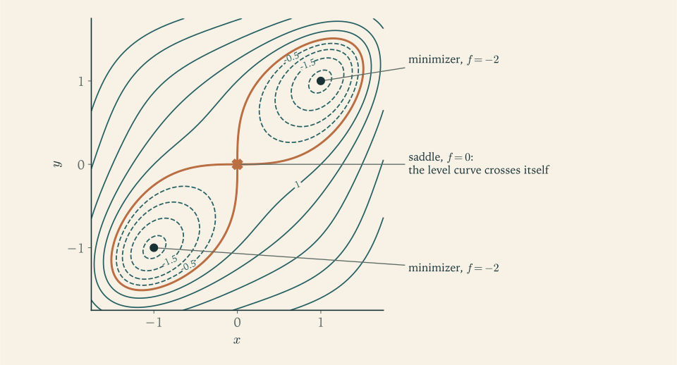
Figure 3.1 shows what the eigenvalues encode. Around a point with positive definite Hessian the level sets are nested closed curves, nearly ellipses, shrinking to the point. Around a saddle the level set through the point consists of two crossing curves, and the four sectors between them alternate between higher and lower values.
Common mistake. Equating a stationary point with a minimizer. A student solves \(\nabla f=0\) for \(f(x,y)=x^2-4xy+y^2\) , finds the origin, notes that both pure second derivatives equal \(2\) , and reports a minimum. The Hessian \(\begin{pmatrix}2&-4\\-4&2\end{pmatrix}\) has eigenvalues \(-2\) and \(6\) , the origin is a saddle, and \(f(1,1)=-2<0\) . Classify curvature with eigenvalues, not with diagonal entries; treat a positive definite Hessian as a local statement; and claim a global minimum only after proving convexity on the whole domain or after an existence-and-comparison argument like that of Example 3.6.
Everything in this chapter assumed that no constraint is active at the solution. When the feasible set has a boundary and the solution sits on it, the gradient of the objective does not vanish, as Example 1.5 showed. The next three chapters develop the theory for that case, beginning with the problems whose constraints and objectives are simplest: linear and quadratic programs.
Exercises
-
Find the stationary point of \(f(x,y)=x^2+xy+y^2-3x\) , classify it using the eigenvalues of the Hessian, and state whether it is a global minimizer, citing the theorem that justifies your answer.
Answer
\(\nabla f=(2x+y-3,\ x+2y)\) vanishes only at \((2,-1)\) , where \(f=-3\) . The Hessian \(\begin{pmatrix}2&1\\1&2\end{pmatrix}\) is constant with eigenvalues \(1\) and \(3\) , so \(f\) is convex on \(\mathbb R^2\) (Theorem 2.6) and the stationary point is the global minimizer (Theorem 3.5); it is unique because \(f\) is strongly convex.
-
Find and classify all stationary points of \(f(x,y)=x^3+y^3-3xy\) , and decide whether \(f\) has a global minimizer on \(\mathbb R^2\) .
Solution
The gradient is \((3x^2-3y,\ 3y^2-3x)\) . It vanishes when \(y=x^2\) and \(x=y^2\) . Substituting the first into the second gives \(x=x^4\) , so \(x(x^3-1)=0\) and, over the reals, \(x=0\) or \(x=1\) . The stationary points are \((0,0)\) and \((1,1)\) .
The Hessian is
\[ \nabla^2f(x,y)=\begin{pmatrix}6x&-3\\-3&6y\end{pmatrix}. \]At \((0,0)\) it is \(\begin{pmatrix}0&-3\\-3&0\end{pmatrix}\) with eigenvalues \(3\) and \(-3\) . A negative eigenvalue excludes a local minimizer by Theorem 3.3, and the positive eigenvalue excludes a local maximizer by the same theorem applied to \(-f\) ; the origin is a saddle point with \(f=0\) . At \((1,1)\) the Hessian is \(\begin{pmatrix}6&-3\\-3&6\end{pmatrix}\) with eigenvalues \(3\) and \(9\) , both positive, so by Theorem 3.4 the point is a strict local minimizer, with \(f(1,1)=1+1-3=-1\) .
There is no global minimizer: \(f(x,0)=x^3\to-\infty\) as \(x\to-\infty\) , so \(p^\star=-\infty\) . The local minimizer \((1,1)\) is the best point in its neighbourhood only.
-
Let \(f(x,y)=(y-x^2)(y-2x^2)\) . Show that for every direction \(d\ne 0\) the one-variable function \(t\mapsto f(td)\) has a strict local minimum at \(t=0\) , and yet the origin is not a local minimizer of \(f\) ; diagnose what is wrong with inferring local minimality from behaviour along lines.
Solution
Expand: \(f(x,y)=y^2-3x^2y+2x^4\) . Take a direction \(d=(a,b)\ne 0\) and let \(g(t)=f(ta,tb)=b^2t^2-3a^2b\,t^3+2a^4t^4\) .
If \(b\ne 0\) , then \(g(t)=t^2\bigl(b^2-3a^2bt+2a^4t^2\bigr)\) , and the bracket tends to \(b^2>0\) as \(t\to 0\) , so \(g(t)>0=g(0)\) for all small \(t\ne 0\) . If \(b=0\) , then \(a\ne 0\) and \(g(t)=2a^4t^4>0\) for \(t\ne 0\) . In every direction, \(t=0\) is a strict local minimum of \(g\) .
Nevertheless the origin is not a local minimizer of \(f\) . Along the parabola \(y=\tfrac32x^2\) ,
\[ f\bigl(x,\tfrac32x^2\bigr)=\bigl(\tfrac12x^2\bigr)\bigl(-\tfrac12x^2\bigr)=-\tfrac14x^4<0\qquad\text{for }x\ne 0, \]and such points lie arbitrarily close to the origin. The function is negative exactly in the thin region between the parabolas \(y=x^2\) and \(y=2x^2\) . Every line through the origin leaves that region near the origin, which is why each line sees a minimum, but the interval of \(t\) on which \(g\) is positive shrinks to nothing as the direction approaches the \(x\) -axis, so no single ball works for all directions. Local minimality requires one neighbourhood valid in all directions simultaneously. The second-order test is consistent with this: the Hessian at the origin is diagonal with entries \(0\) and \(2\) , positive semidefinite and singular, so Theorem 3.4 does not apply.
-
State and prove the analogues of Theorems 3.1 and 3.3 for a local maximizer by applying those theorems to \(-f\) , and explain why a stationary point whose Hessian has both a positive and a negative eigenvalue must be a saddle point.
Hint
A local maximizer of \(f\) is a local minimizer of \(-f\) , whose gradient is \(-\nabla f\) and whose Hessian is \(-\nabla^2f\) . So the gradient vanishes and the Hessian is negative semidefinite. If the Hessian has a positive eigenvalue it is not negative semidefinite, and if it has a negative one it is not positive semidefinite; then both kinds of local extremum are excluded.
-
Let \(f\) be convex and differentiable on \(\mathbb R^n\) . Prove that the set of stationary points of \(f\) is convex, and that if \(x\) and \(y\) are two distinct stationary points then \(f\) is constant on the segment joining them.
Solution
By Theorem 3.5 with \(C=\mathbb R^n\) , a point is stationary if and only if it is a global minimizer. So the set of stationary points is the set of global minimizers, which is either empty, and then trivially convex, or equal to the sublevel set \(\{x:f(x)\le p^\star\}\) , which is convex by Proposition 2.4. This proves the first claim.
For the second, let \(x\ne y\) be stationary. Both are global minimizers, so \(f(x)=f(y)=p^\star\) . For \(\theta\in[0,1]\) the point \(z=\theta x+(1-\theta)y\) satisfies \(f(z)\le\theta f(x)+(1-\theta)f(y)=p^\star\) by convexity and \(f(z)\ge p^\star\) because \(p^\star\) is the minimum value. Hence \(f(z)=p^\star\) for every point of the segment. A consequence worth noting: a convex function cannot have two isolated stationary points, which is one way to see at a glance that the function of Example 3.6 is not convex.
-
For \(f(x)=x_1^2+x_1x_2+x_2^2-3x_1\) and the point \(x=(0,0)\) , compute \(\nabla f(x)\) and the modulus \(m\) , use Proposition 3.6 to bound \(f(x)-f^\star\) and \(\lVert x-x^\star\rVert\) from above, and compare both bounds with the true values.
Solution
The gradient is \(\nabla f(x)=(2x_1+x_2-3,\ x_1+2x_2)\) , so \(\nabla f(0,0)=(-3,0)\) and \(\lVert\nabla f(0,0)\rVert^2=9\) . The Hessian has eigenvalues \(1\) and \(3\) , so \(m=1\) . Proposition 3.6 gives
\[ f(x)-f^\star\le\frac{9}{2\cdot 1}=4.5,\qquad\lVert x-x^\star\rVert\le\frac{3}{1}=3 . \]From Example 3.4, \(x^\star=(2,-1)\) and \(f^\star=-3\) . Since \(f(0,0)=0\) , the true gap is \(3\le 4.5\) , and the true distance is \(\lVert(2,-1)\rVert=\sqrt5\approx 2.236\le 3\) . The lower bound of the proposition also holds: \(\tfrac m2\lVert x-x^\star\rVert^2=2.5\le 3\) . The upper bounds are not tight here because the gradient \((-3,0)\) is not an eigenvector for the smallest eigenvalue; the bound is attained only when the error \(x-x^\star\) lies along the direction of weakest curvature.
-
For \(P=\begin{pmatrix}2&-1\\-1&2\end{pmatrix}\) and \(q=(-1,-4)\) , find the minimizer and minimum value of \(\tfrac12x^{\top}Px+q^{\top}x\) , and verify the identity of Theorem 3.7(a) at \(x=0\) .
Answer
Solving \(2x_1-x_2=1\) and \(-x_1+2x_2=4\) gives \(x^\star=(2,3)\) , and \(f(x^\star)=\tfrac12q^{\top}x^\star=\tfrac12(-2-12)=-7\) . At \(x=0\) : \(f(0)-f(x^\star)=7\) and \(\tfrac12x^{\star\top}Px^\star=\tfrac12(8-12+18)=7\) .
-
For each quadratic \(\tfrac12x^{\top}Px+q^{\top}x\) decide which case of Theorem 3.7 applies, and give the minimizers and minimum value or a direction of unbounded descent: (a) \(P=\begin{pmatrix}1&2\\2&4\end{pmatrix}\) , \(q=(1,2)\) ; (b) the same \(P\) with \(q=(1,0)\) ; (c) \(P=\begin{pmatrix}1&2\\2&1\end{pmatrix}\) , \(q=(0,0)\) .
Solution
(a) The eigenvalues of \(P\) are \(0\) and \(5\) (trace \(5\) , determinant \(0\) ), so \(P\succeq 0\) is singular with null space spanned by \((2,-1)\) . Since \(q^{\top}(2,-1)=2-2=0\) , the vector \(q\) is orthogonal to the null space and so lies in the range of \(P\) . Case (b) of Theorem 3.7 with a solvable system: \(Px=-q\) reads \(x_1+2x_2=-1\) (twice). Writing \(u=x_1+2x_2\) , the function is \(\tfrac12u^2+u\) , so the minimum value is \(\tfrac12-1=-\tfrac12\) , attained on the whole line \(x_1+2x_2=-1\) .
(b) Now \(q^{\top}(2,-1)=2\ne 0\) , so \(q\) is not in the range of \(P\) . Along the null direction \(d=(-2,1)\) the quadratic term vanishes and \(f(td)=tq^{\top}d=-2t\to-\infty\) . The function is unbounded below.
(c) The eigenvalues are \(1-2=-1\) and \(1+2=3\) . Case (c): along the eigenvector \((1,-1)\) for \(-1\) , \(f(t,-t)=\tfrac12(t^2-4t^2+t^2)=-t^2\to-\infty\) . Unbounded below, even though both diagonal entries of \(P\) are positive.
-
Fit the line \(y=c_0+c_1t\) to the four points \((t,y)=(-1,0),(0,1),(1,1),(2,4)\) by solving the normal equations, and verify that the residual is orthogonal to both columns of \(A\) .
Solution
With rows \((1,t_i)\) ,
\[ A=\begin{pmatrix}1&-1\\1&0\\1&1\\1&2\end{pmatrix},\quad b=\begin{pmatrix}0\\1\\1\\4\end{pmatrix},\quad A^{\top}A=\begin{pmatrix}4&2\\2&6\end{pmatrix},\quad A^{\top}b=\begin{pmatrix}6\\9\end{pmatrix}. \]The normal equations are \(4c_0+2c_1=6\) and \(2c_0+6c_1=9\) . Doubling the second and subtracting the first gives \(10c_1=12\) , so \(c_1=1.2\) and then \(c_0=(6-2.4)/4=0.9\) . The fitted line is \(y=0.9+1.2t\) .
The fitted values are \(-0.3,\ 0.9,\ 2.1,\ 3.3\) and the residual is \(b-Ax^\star=(0.3,\ 0.1,\ -1.1,\ 0.7)\) . Orthogonality to the first column: \(0.3+0.1-1.1+0.7=0\) . Orthogonality to the second column: \(-0.3+0-1.1+1.4=0\) . The columns of \(A\) are independent, so \(A^{\top}A\) is positive definite and this is the unique minimizer; the minimum value is the squared residual norm \(0.09+0.01+1.21+0.49=1.8\) .
-
Derive \(\nabla f(x)=2A^{\top}(Ax-b)\) for \(f(x)=\lVert Ax-b\rVert^2\) by expanding \(f(x+d)-f(x)\) and identifying the term linear in \(d\) , and prove that \(A^{\top}A\) is positive definite if and only if the columns of \(A\) are linearly independent.
Hint
Expand \(\lVert A(x+d)-b\rVert^2=\lVert Ax-b\rVert^2+2(Ax-b)^{\top}Ad+\lVert Ad\rVert^2\) ; the middle term is \(\bigl(2A^{\top}(Ax-b)\bigr)^{\top}d\) and the last is of second order. For definiteness use \(d^{\top}A^{\top}Ad=\lVert Ad\rVert^2\) , which is zero exactly when \(Ad=0\) .
-
A student minimizing \(f(x,y)=x^2-4xy+y^2\) finds the stationary point \((0,0)\) , observes that both pure second partial derivatives equal \(2\) , and concludes that the origin is a minimizer. Identify the error, classify the point correctly, and exhibit a point where \(f\) is negative.
Answer
Pure second derivatives are curvatures along the axes only. The Hessian \(\begin{pmatrix}2&-4\\-4&2\end{pmatrix}\) has eigenvalues \(-2\) and \(6\) , so the origin is a saddle point. For instance \(f(1,1)=1-4+1=-2<0=f(0,0)\) .
-
Find all stationary points of \(f(x,y)=(x^2-1)^2+y^2\) , classify each, identify the global minimizers, and explain why a global minimizer was guaranteed to exist before any computation.
Answer
\(\nabla f=(4x(x^2-1),\ 2y)\) vanishes at \((0,0)\) , \((1,0)\) , \((-1,0)\) . The Hessian is diagonal with entries \(12x^2-4\) and \(2\) : at the origin the entries are \(-4\) and \(2\) , a saddle with \(f=1\) ; at \((\pm1,0)\) they are \(8\) and \(2\) , strict local minimizers with \(f=0\) . Since \(f\ge 0\) everywhere, both are global minimizers. Existence was guaranteed because \(f\) is continuous and coercive.
-
Let \(f\) be twice continuously differentiable with \(\nabla f(x^\star)=0\) and \(\nabla^2f(x)\succeq 0\) for every \(x\) in some open ball centred at \(x^\star\) . Prove that \(x^\star\) is a local minimizer, and use \(f(x)=x^3\) to show that positive semidefiniteness at the single point \(x^\star\) would not suffice.
Solution
Let \(B\) be the open ball on which the Hessian is positive semidefinite. A ball is an open convex set, so by Theorem 2.6 the function \(f\) is convex on \(B\) . Since \(\nabla f(x^\star)=0\) and \(x^\star\in B\) , Theorem 3.5 with \(C=B\) shows that \(x^\star\) is a global minimizer of \(f\) over \(B\) . A point that minimizes \(f\) over a ball centred at itself is, by Definition 1.3, a local minimizer of \(f\) .
For \(f(x)=x^3\) we have \(f'(0)=0\) and \(f''(0)=0\) , which is positive semidefinite, but \(f''(x)=6x<0\) for every \(x<0\) , so the hypothesis fails on every ball about \(0\) , and indeed \(f(x)<0=f(0)\) for \(x<0\) . The difference between the two situations is the difference between knowing curvature at one point and knowing it throughout a neighbourhood: only the latter gives convexity, and convexity is what turns stationarity into minimality. Note that the conclusion here is a local minimizer, not necessarily a strict one; \(f\equiv 0\) satisfies the hypotheses.
-
For the family \(f_c(x,y)=x^2+cxy+y^2+x\) with real parameter \(c\) , determine for which \(c\) there is a unique minimizer and find it as a function of \(c\) ; then describe what happens at \(c=2\) and for \(c>2\) .
Answer
The Hessian \(\begin{pmatrix}2&c\\c&2\end{pmatrix}\) is positive definite exactly when \(\lvert c\rvert<2\) ; then the unique minimizer solves \(2x+cy=-1\) , \(cx+2y=0\) , giving \(x=-2/(4-c^2)\) and \(y=c/(4-c^2)\) . At \(c=2\) , \(f=(x+y)^2+x\) and along \((t,-t)\) the value is \(t\) , unbounded below as \(t\to-\infty\) : case (b) of Theorem 3.7 with \(q=(1,0)\) outside the range of \(P\) . For \(c>2\) the Hessian has the negative eigenvalue \(2-c\) and \(f\) is unbounded below by case (c).
-
Let \(\mu>0\) . Use Theorems 1.4 and 3.5 to prove that \(f(x)=\lVert Ax-b\rVert^2+\mu\lVert x\rVert^2\) has exactly one minimizer for every matrix \(A\) , show that it solves \((A^{\top}A+\mu I)x=A^{\top}b\) , and compute it for \(A=\begin{pmatrix}1&1\end{pmatrix}\) , \(b=2\) , \(\mu=1\) .
Solution
The function is continuous and \(f(x)\ge\mu\lVert x\rVert^2\) , so it is coercive on \(\mathbb R^n\) and Theorem 1.4 gives a minimizer. Its Hessian is \(2A^{\top}A+2\mu I\) . For any \(d\) , \(d^{\top}(2A^{\top}A+2\mu I)d=2\lVert Ad\rVert^2+2\mu\lVert d\rVert^2\ge 2\mu\lVert d\rVert^2\) , so the Hessian is positive definite everywhere, \(f\) is strictly (indeed \(2\mu\) -strongly) convex, and by Theorem 2.10 the minimizer is unique. No assumption on the rank of \(A\) was needed; the added term supplies the curvature that \(A^{\top}A\) may lack.
By Theorem 3.5 the minimizer is the solution of \(\nabla f(x)=2A^{\top}(Ax-b)+2\mu x=0\) , that is, \((A^{\top}A+\mu I)x=A^{\top}b\) . For \(A=\begin{pmatrix}1&1\end{pmatrix}\) , \(b=2\) , \(\mu=1\) :
\[ A^{\top}A+I=\begin{pmatrix}2&1\\1&2\end{pmatrix},\qquad A^{\top}b=\begin{pmatrix}2\\2\end{pmatrix},\qquad x^\star=\begin{pmatrix}2/3\\2/3\end{pmatrix}. \]The value is \((\tfrac43-2)^2+\tfrac89=\tfrac49+\tfrac89=\tfrac43\) . Without the penalty the problem would have a whole line of minimizers \(x_1+x_2=2\) ; the penalty selects a single point, pulled toward the origin.
-
Given points \(a_1,a_2,a_3\in\mathbb R^n\) , show that \(f(x)=\sum_{i=1}^{3}\lVert x-a_i\rVert^2\) is minimized at the centroid \(\bar a=\tfrac13(a_1+a_2+a_3)\) and that \(f(x)=3\lVert x-\bar a\rVert^2+f(\bar a)\) for every \(x\) .
Hint
The gradient is \(2\sum_i(x-a_i)=6x-2(a_1+a_2+a_3)\) and the Hessian is \(6I\) . For the identity write \(x-a_i=(x-\bar a)+(\bar a-a_i)\) , expand the squares, and use \(\sum_i(\bar a-a_i)=0\) to kill the cross terms.
-
For the function \(f(x,y)=(1-x)^2+100(y-x^2)^2\) show that \((1,1)\) is the only stationary point and is the global minimizer, compute the Hessian there, and find the ratio of its largest to its smallest eigenvalue.
Answer
\(\nabla f=(-2(1-x)-400x(y-x^2),\ 200(y-x^2))\) . The second component forces \(y=x^2\) , and then the first forces \(x=1\) , so \((1,1)\) is the only stationary point; since \(f\ge 0=f(1,1)\) it is the global minimizer. The Hessian there is \(\begin{pmatrix}802&-400\\-400&200\end{pmatrix}\) with eigenvalues \(501\pm\sqrt{250601}\) , approximately \(1001.6\) and \(0.399\) ; their ratio is about \(2508\) .
-
Theorem 3.5 has two hypotheses beyond differentiability: convexity of \(f\) and openness of \(C\) . For each, give a one-variable example showing that the conclusion fails when that hypothesis alone is dropped.
Answer
Convexity dropped: \(f(x)=-x^2\) on \(C=\mathbb R\) has \(f'(0)=0\) , but \(0\) is the global maximizer. Openness dropped: the convex function \(f(x)=x\) on \(C=[0,1]\) is minimized at \(x=0\) , where \(f'(0)=1\ne 0\) .