The proof of Theorem 3.1 contained an algorithm in disguise: wherever the gradient is not zero, a small enough step against it lowers the function. Repeating that step is the oldest and most widely used method of continuous optimization. Two questions decide whether it is any good. How small is “small enough”, and can the step length be chosen without trial and error? And how many steps are needed to reach a given accuracy, as a function of quantities one can know in advance?
On \(f(x)=\tfrac52x^2\) the answers can be read off. The step \(x-\alpha f'(x)=(1-5\alpha)x\) multiplies the current point by a fixed factor. With \(\alpha=0.2\) the factor is \(0\) and the method lands on the minimizer at once; with \(\alpha=0.3\) the factor is \(-0.5\) and the iterates alternate in sign while halving; with \(\alpha=0.5\) the factor is \(-1.5\) and they grow without bound. The same step length that is too timid for one function is disastrous for another. This chapter identifies the single constant, the Lipschitz constant \(L\) of the gradient, that separates safe steps from unsafe ones, and proves three rates of convergence, each under its own hypotheses.
7.1 The method and the choice of step
Definition 7.1 (descent direction, gradient method). Let \(f\) be differentiable at \(x\) . A vector \(d\) is a descent direction at \(x\) if \(\nabla f(x)^{\top}d<0\) . The gradient method with step sizes \(\alpha_k>0\) generates, from a starting point \(x_0\) , the iterates
Along a descent direction the function decreases initially, since the derivative of \(t\mapsto f(x+td)\) at \(t=0\) is \(\nabla f(x)^{\top}d\) . Among unit vectors the negative normalised gradient gives the most negative such derivative, by the Cauchy–Schwarz inequality, which is why the method is also called steepest descent. The step size, sometimes called the learning rate, is the only free choice. Three rules are common. A constant step uses the same \(\alpha\) throughout. Exact line search chooses \(\alpha_k\) to minimize \(f(x_k-\alpha\nabla f(x_k))\) over \(\alpha>0\) . Backtracking starts from a trial step and shrinks it until a sufficient-decrease test is passed. We analyse the constant step first, because the analysis reveals what the other rules are estimating.
7.2 Smoothness and the descent lemma
Definition 7.2 (smoothness). A differentiable function \(f:\mathbb R^n\to\mathbb R\) is \(L\) -smooth if its gradient is Lipschitz continuous with constant \(L\) :
Smoothness limits how fast the gradient can turn. It is an upper bound on curvature, complementary to the lower bound that strong convexity provides. If \(f\) is twice continuously differentiable and every eigenvalue of every Hessian \(\nabla^2f(z)\) lies in \([-L,L]\) , then \(f\) is \(L\) -smooth: by the fundamental theorem of calculus applied to \(t\mapsto\nabla f(x+t(y-x))\) ,
and the integrand has norm at most \(L\lVert y-x\rVert\) . For a convex function the Hessian eigenvalues are nonnegative, so the condition is simply \(\nabla^2f(z)\preceq LI\) . A quadratic \(\tfrac12x^{\top}Px+q^{\top}x\) with \(P\succeq 0\) is \(L\) -smooth with \(L\) the largest eigenvalue of \(P\) .
Lemma 7.3 (descent lemma). If \(f\) is \(L\) -smooth, then for all \(x,y\in\mathbb R^n\) ,
Proof. Let \(\phi(t)=f(x+t(y-x))\)
for \(t\in[0,1]\)
, so that \(\phi'(t)=\nabla f(x+t(y-x))^{\top}(y-x)\)
. The fundamental theorem of calculus (math.calculus.fundamental-theorem-bridge) gives \(f(y)-f(x)=\phi(1)-\phi(0)=\int_0^1\phi'(t)\,dt\)
. Subtract and add the constant \(\nabla f(x)^{\top}(y-x)\)
:
By the Cauchy–Schwarz inequality and then smoothness, the integrand is at most \(\lVert\nabla f(x+t(y-x))-\nabla f(x)\rVert\,\lVert y-x\rVert\le Lt\lVert y-x\rVert^2\) . Integrating \(Lt\lVert y-x\rVert^2\) over \([0,1]\) gives \(\tfrac L2\lVert y-x\rVert^2\) .
Compare the lemma with Theorem 2.5. A convex function lies above each of its tangent planes; an \(L\) -smooth function lies below each tangent plane plus a fixed paraboloid. A function that is both is trapped between the two, and the trap is what makes the method analysable: the right side of the lemma is a quadratic upper model of \(f\) around \(x\) , valid everywhere, and a gradient step is exactly a move toward the minimizer of that model.
7.3 Guaranteed decrease
Theorem 7.4 (one-step decrease). Let \(f\) be \(L\) -smooth and let \(x^+=x-\alpha\nabla f(x)\) with \(\alpha>0\) . Then
In particular \(f(x^+)<f(x)\) whenever \(0<\alpha<2/L\) and \(\nabla f(x)\ne 0\) , and for \(\alpha=1/L\) ,
Proof. Apply Lemma 7.3 with \(y=x^+\) , so \(y-x=-\alpha\nabla f(x)\) : the linear term is \(-\alpha\lVert\nabla f(x)\rVert^2\) and the quadratic term is \(\tfrac L2\alpha^2\lVert\nabla f(x)\rVert^2\) . The factor \(\alpha(1-\alpha L/2)\) is positive exactly for \(0<\alpha<2/L\) and is largest, equal to \(1/(2L)\) , at \(\alpha=1/L\) .
The theorem needs no convexity. It says that \(1/L\) is the step that minimizes the upper model, and that any step below \(2/L\) still makes progress. Summing the guaranteed decreases gives the only conclusion available for general smooth functions.
Corollary 7.5 (gradients become small). Let \(f\) be \(L\) -smooth and bounded below by \(f_{\inf}\) , and run the gradient method with \(\alpha=1/L\) . Then for every \(k\ge 1\) ,
and \(\nabla f(x_k)\to 0\) .
Proof. By Theorem 7.4, \(\tfrac1{2L}\lVert\nabla f(x_i)\rVert^2\le f(x_i)-f(x_{i+1})\) . Summing over \(i=0,\dots,k-1\) telescopes the right side to \(f(x_0)-f(x_k)\le f(x_0)-f_{\inf}\) . The smallest of \(k\) nonnegative terms is at most their average, which gives the bound; and since the series \(\sum_i\lVert\nabla f(x_i)\rVert^2\) has bounded partial sums, its terms tend to zero.
For a nonconvex function this is all that can be promised: the method drives the gradient to zero, so every limit point of the iterates is a stationary point. Whether that point is a minimizer, a saddle, or even a maximizer is not decided by the corollary, and Chapter 3 explained why no first-order information could decide it.
Example 7.1: Three steps on a scalar quadratic
For \(f(x)=\tfrac52x^2\) the derivative is \(5x\) , and \(\lvert5x-5y\rvert=5\lvert x-y\rvert\) , so \(L=5\) . A gradient step gives \(x^+=(1-5\alpha)x\) , hence \(x_k=(1-5\alpha)^kx_0\) .
With \(\alpha=1/L=0.2\) the factor is \(0\) : the minimizer is reached in one step, because for a one-variable quadratic the upper model of Lemma 7.3 is the function itself. With \(\alpha=0.3\) the factor is \(-0.5\) : from \(x_0=1\) the iterates are \(1,-0.5,0.25,-0.125\) , overshooting the minimizer each time but converging. With \(\alpha=0.5\) the factor is \(-1.5\) : the iterates \(1,-1.5,2.25,-3.375\) diverge, and \(f\) increases at every step. The threshold between the last two behaviours is \(\lvert1-5\alpha\rvert=1\) , that is, \(\alpha=2/L=0.4\) , where the iterates oscillate between \(x_0\) and \(-x_0\) forever.
Theorem 7.4 predicts all of this. Its decrease factor \(\alpha(1-\alpha L/2)\) equals \(0.1\) at \(\alpha=0.2\) , equals \(0.075\) at \(\alpha=0.3\) , vanishes at \(\alpha=0.4\) , and is negative at \(\alpha=0.5\) , where the bound permits an increase and an increase occurs.
7.4 Convex functions: a sublinear rate
Corollary 7.5 controls gradients. When \(f\) is convex, the same step controls function values.
Theorem 7.6 (rate for smooth convex functions). Let \(f\) be convex and \(L\) -smooth with a minimizer \(x^\star\) , and let \(f^\star=f(x^\star)\) . The gradient method with \(\alpha=1/L\) satisfies, for every \(k\ge 1\) ,
Proof. Write \(x\) for an iterate, \(g=\nabla f(x)\) , and \(x^+=x-g/L\) . Theorem 7.4 gives \(f(x^+)\le f(x)-\tfrac1{2L}\lVert g\rVert^2\) . Convexity, in the form of Theorem 2.5 with base point \(x\) evaluated at \(x^\star\) , gives \(f(x)\le f^\star+g^{\top}(x-x^\star)\) . Combining,
The right side is a difference of squares in disguise. Expanding \(\lVert x^+-x^\star\rVert^2=\lVert x-x^\star\rVert^2-\tfrac2Lg^{\top}(x-x^\star)+\tfrac1{L^2}\lVert g\rVert^2\) and rearranging,
Hence \(f(x_{i+1})-f^\star\le\tfrac L2\bigl(\lVert x_i-x^\star\rVert^2-\lVert x_{i+1}-x^\star\rVert^2\bigr)\) for every \(i\) . Sum over \(i=0,\dots,k-1\) ; the right side telescopes to at most \(\tfrac L2\lVert x_0-x^\star\rVert^2\) . The values \(f(x_i)\) are nonincreasing by Theorem 7.4, so each of the \(k\) terms on the left is at least \(f(x_k)-f^\star\) , and therefore \(k\,(f(x_k)-f^\star)\le\tfrac L2\lVert x_0-x^\star\rVert^2\) .
Two by-products of the proof are worth recording. The key inequality shows that \(\lVert x_{i+1}-x^\star\rVert\le\lVert x_i-x^\star\rVert\) : the iterates never move away from a minimizer. And the rate \(1/k\) is called sublinear: to halve the guaranteed error one must double the number of iterations, and accuracy \(\varepsilon\) needs on the order of \(L\lVert x_0-x^\star\rVert^2/\varepsilon\) steps.
Example 7.2: A smooth convex function that is not quadratic
Let \(f(x)=\log(1+e^{x})-0.3x\) on \(\mathbb R\) . With \(\sigma(x)=e^{x}/(1+e^{x})\) , the derivatives are \(f'(x)=\sigma(x)-0.3\) and \(f''(x)=\sigma(x)(1-\sigma(x))\) . Since \(0<\sigma<1\) , the second derivative lies in \((0,\tfrac14]\) , so \(f\) is convex and \(L\) -smooth with \(L=\tfrac14\) (Exercise 2.14). The minimizer solves \(\sigma(x)=0.3\) , that is, \(x^\star=\log(3/7)\approx-0.8473\) .
The step \(\alpha=1/L=4\) gives the iteration \(x_{k+1}=x_k-4(\sigma(x_k)-0.3)\) . From \(x_0=2\) :
The errors \(f(x_k)-f^\star\) are approximately \(0.916\) , \(0.0306\) , \(2.1\times10^{-4}\) , \(4.8\times10^{-6}\) for \(k=0,1,2,3\) . Theorem 7.6 guarantees \(f(x_k)-f^\star\le\tfrac18(2-x^\star)^2/k\approx1.013/k\) , that is, \(1.013\) , \(0.507\) , \(0.338\) for \(k=1,2,3\) . The guarantee holds, with a great deal to spare.
Why is the method so much faster than its guarantee here? The function is not strongly convex on \(\mathbb R\) , because \(f''(x)\to 0\) as \(\lvert x\rvert\to\infty\) , so only the sublinear theorem applies globally. But near \(x^\star\) the curvature is \(f''(x^\star)=0.3\cdot0.7=0.21>0\) , and once the iterates are close the behaviour is that of a strongly convex function, with the error shrinking by a roughly constant factor per step. The theorem is a worst-case bound over all smooth convex functions, including ones that are nearly flat around their minimizers.
7.5 Strong convexity, linear convergence, and conditioning
Theorem 7.7 (rate for smooth strongly convex functions). Let \(f\) be \(m\) -strongly convex and \(L\) -smooth, with minimizer \(x^\star\) . The gradient method with \(\alpha=1/L\) satisfies
Proof. With the notation of the previous proof, expand
Two inequalities bound the last two terms. First, strong convexity (Proposition 2.9 with base point \(x\) , evaluated at \(x^\star\) ) gives \(f^\star\ge f(x)+g^{\top}(x^\star-x)+\tfrac m2\lVert x-x^\star\rVert^2\) , that is,
Second, Theorem 7.4 gives \(f^\star\le f(x^+)\le f(x)-\tfrac1{2L}\lVert g\rVert^2\) , that is, \(\lVert g\rVert^2\le 2L\,(f(x)-f^\star)\) . Substituting both,
Applying this \(k\) times gives the first claim. For the second, Lemma 7.3 with base point \(x^\star\) , where the gradient vanishes, gives \(f(x_k)-f^\star\le\tfrac L2\lVert x_k-x^\star\rVert^2\) .
The error is multiplied by a fixed factor below one at every step. This is linear convergence: the number of correct digits grows in proportion to the number of iterations. The factor depends only on the ratio
the condition number of the problem. Since \((1-1/\kappa)^k\le e^{-k/\kappa}\) , reducing the squared error by a factor \(\varepsilon\) takes at most \(\kappa\log(1/\varepsilon)\) iterations. A well-conditioned problem, with \(\kappa\) near \(1\) , is solved in a handful of steps; a problem with \(\kappa=10^4\) needs tens of thousands. The inequality \(m\le L\) always holds, by comparing the lower bound of Proposition 2.9 with the upper bound of Lemma 7.3.
For quadratic functions the behaviour can be computed exactly, and the computation shows where the condition number comes from.
Proposition 7.8 (gradient method on a quadratic). Let \(f(x)=\tfrac12x^{\top}Px+q^{\top}x\) with \(P\succ 0\) , smallest eigenvalue \(m\) , largest eigenvalue \(L\) , and minimizer \(x^\star\) . For a constant step \(\alpha\) the errors satisfy \(x_{k+1}-x^\star=(I-\alpha P)(x_k-x^\star)\) . In an orthonormal basis of eigenvectors of \(P\) , the component of the error along an eigenvector with eigenvalue \(\mu\) is multiplied by \(1-\alpha\mu\) at each step. The method converges from every starting point if and only if \(0<\alpha<2/L\) , and the worst-case contraction factor \(\max\{\lvert1-\alpha m\rvert,\lvert1-\alpha L\rvert\}\) is smallest for
Proof. Since \(\nabla f(x)=Px+q=P(x-x^\star)\) , we have \(x_{k+1}-x^\star=x_k-x^\star-\alpha P(x_k-x^\star)\) . If \(Pv=\mu v\) then \((I-\alpha P)v=(1-\alpha\mu)v\) , which gives the statement about components. Every component tends to zero if and only if \(\lvert1-\alpha\mu\rvert<1\) for every eigenvalue \(\mu\in[m,L]\) , that is, \(0<\alpha\mu<2\) for all of them, that is, \(0<\alpha<2/L\) . The function \(\mu\mapsto\lvert1-\alpha\mu\rvert\) is convex, so its maximum over \([m,L]\) is at an endpoint. As \(\alpha\) increases, \(\lvert1-\alpha m\rvert\) decreases while \(\lvert1-\alpha L\rvert\) eventually increases; the maximum of the two is smallest where \(1-\alpha m=-(1-\alpha L)\) , which gives \(\alpha=2/(m+L)\) and the common value \((L-m)/(L+m)\) .
The proposition explains the slow convergence on ill-conditioned problems as a conflict between directions. A step small enough to be stable in the direction of largest curvature is too small to make progress in the direction of smallest curvature.
Example 7.3: An ill-conditioned quadratic in the plane
Let \(f(x)=\tfrac12(x_1^2+10x_2^2)\) , so \(P\) is diagonal with entries \(1\) and \(10\) : \(m=1\) , \(L=10\) , \(\kappa=10\) , \(x^\star=0\) . Start from \(x_0=(10,1)\) , where \(f=55\) and \(\nabla f=(10,10)\) .
With \(\alpha=1/L=0.1\) the coordinates are multiplied by \(1-0.1=0.9\) and \(1-1=0\) . The steep coordinate \(x_2\) is eliminated at once and the shallow coordinate crawls: \(x_1=(9,0)\) , \(x_2=(8.1,0)\) , \(x_3=(7.29,0)\) , with \(f(x_k)=50\cdot0.81^k\) for \(k\ge 1\) , namely \(40.5\) , \(32.805\) , \(26.572\) . Theorem 7.7 bounds \(\lVert x_k\rVert^2\) by \(0.9^k\cdot101\) , while the actual value is \(100\cdot0.81^k\) ; the bound is valid and somewhat pessimistic.
With \(\alpha=2/(m+L)=2/11\) the multipliers are \(1-\tfrac2{11}=\tfrac9{11}\) and \(1-\tfrac{20}{11}=-\tfrac9{11}\) . Both coordinates now shrink by the same factor \(\tfrac9{11}\approx0.818\) per step, the second with alternating sign: \(x_1\approx(8.18,-0.82)\) , \(x_2\approx(6.69,0.67)\) , \(x_3\approx(5.48,-0.55)\) , and \(f(x_k)=55\,(9/11)^{2k}\) , namely \(36.82\) , \(24.65\) , \(16.50\) . This is faster than the step \(1/L\) , at the price of oscillating across the valley.
To reduce the distance to the minimizer by a factor \(10^{-6}\) requires \(0.9^k\le10^{-6}\) , that is, \(k\ge132\) steps, at \(\alpha=0.1\) , and \((9/11)^k\le10^{-6}\) , that is, \(k\ge69\) steps, at \(\alpha=2/11\) . Either way the count is governed by \(\kappa\) . Compare the sublinear guarantee of Theorem 7.6 for this function, \(505/k\) : at \(k=10\) it gives \(50.5\) , while the true value at \(\alpha=0.1\) is \(50\cdot0.81^{10}\approx6.08\) .
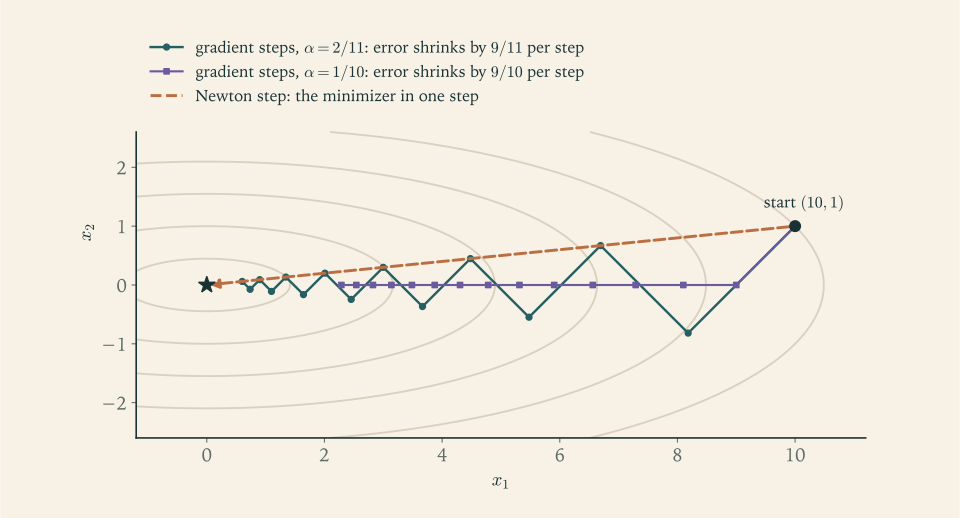
Figure 7.1 shows the geometry behind the algebra. The level curves are ellipses elongated by a factor \(\sqrt{\kappa}\) , and the negative gradient is perpendicular to them, which on a long thin ellipse is nearly perpendicular to the direction of the minimizer. The dashed arrow is the step of the method of the next chapter, which rescales the gradient by the inverse Hessian and so corrects the distortion.
7.6 Choosing the step by line search
In practice \(L\) is rarely known. Exact line search is possible for quadratics, where \(\alpha_k=\lVert g\rVert^2/(g^{\top}Pg)\) with \(g=\nabla f(x_k)\) minimizes \(f\) along the ray, and is usually too expensive otherwise. The standard compromise is to accept any step that achieves a fixed fraction of the decrease predicted by the linear model.
Definition 7.9 (backtracking line search). Fix parameters \(c\in(0,1)\) and \(\beta\in(0,1)\) and an initial trial step \(t_0>0\) . At the point \(x\) with gradient \(g=\nabla f(x)\ne 0\) , set \(t=t_0\) and, while the sufficient-decrease (Armijo) condition
fails, replace \(t\) by \(\beta t\) . Use the first \(t\) that passes as the step size.
Proposition 7.10 (backtracking terminates with a useful step). If \(f\) is \(L\) -smooth, the sufficient-decrease condition holds for every \(t\in(0,\,2(1-c)/L]\) . Consequently backtracking stops after finitely many reductions, with a step \(t\ge\min\{t_0,\ 2\beta(1-c)/L\}\) .
Proof. By Theorem 7.4, \(f(x-tg)\le f(x)-t(1-tL/2)\lVert g\rVert^2\) . The condition is implied whenever \(1-tL/2\ge c\) , that is, \(t\le 2(1-c)/L\) . Backtracking tries \(t_0,\beta t_0,\beta^2t_0,\dots\) ; either \(t_0\) passes, or the first passing trial was preceded by a failing trial \(t/\beta>2(1-c)/L\) .
So backtracking finds, without knowing \(L\) , a step within a constant factor of the theoretically safe range, and the rates of Theorems 7.6 and 7.7 survive with slightly worse constants. It may also accept steps much larger than \(1/L\) where the function happens to be less curved than its worst case.
Example 7.4: Backtracking on the same quadratic
Take \(f(x)=\tfrac12(x_1^2+10x_2^2)\) at \(x=(10,1)\) , with \(g=(10,10)\) , \(\lVert g\rVert^2=200\) , \(f(x)=55\) , and parameters \(c=0.25\) , \(\beta=0.5\) , \(t_0=1\) .
Trial \(t=1\) : the point is \((0,-9)\) with \(f=405\) ; the test requires \(f\le55-50=5\) . Fail. Trial \(t=0.5\) : the point is \((5,-4)\) with \(f=12.5+80=92.5\) ; the test requires \(f\le55-25=30\) . Fail. Trial \(t=0.25\) : the point is \((7.5,-1.5)\) with \(f=28.125+11.25=39.375\) ; the test requires \(f\le55-12.5=42.5\) . Pass.
The accepted step \(0.25\) is larger than \(1/L=0.1\) , even larger than \(2/L=0.2\) , and it gives a lower value, \(39.375\) , than the step \(1/L\) gave in Example 7.3, \(40.5\) . Proposition 7.10 guaranteed acceptance for any \(t\le2(1-c)/L=0.15\) , hence an accepted step of at least \(0.075\) ; the search did better than its guarantee because from this particular point a longer step is still profitable.
7.7 What a small gradient certifies
The gradient method produces a sequence, and at some point it must be stopped. The usual rule stops when \(\lVert\nabla f(x_k)\rVert\le\varepsilon\) . What that implies depends on the class of the function. If \(f\) is \(m\) -strongly convex, Proposition 3.6 turns the gradient norm into a certificate: \(f(x_k)-f^\star\le\varepsilon^2/(2m)\) and \(\lVert x_k-x^\star\rVert\le\varepsilon/m\) . If \(f\) is merely convex, a small gradient bounds the error only through \(f(x_k)-f^\star\le\lVert\nabla f(x_k)\rVert\,\lVert x_k-x^\star\rVert\) , which requires knowing how far away the minimizer might be. If \(f\) is not convex, a small gradient says that the point is nearly stationary, and nothing about optimality.
Example 7.5: The same gradient norm, three meanings
At \(x=(1,0.01)\) the function of Example 7.3 has \(\nabla f=(1,0.1)\) and \(\lVert\nabla f\rVert^2=1.01\) . With \(m=1\) , Proposition 3.6 certifies \(f(x)-f^\star\le1.01/2=0.505\) ; the true gap is \(f(x)=0.5+0.0005=0.5005\) . The certificate is nearly tight because the error lies almost entirely in the direction of smallest curvature.
For \(f(x)=e^{x}\) at \(x=-10\) the derivative is \(e^{-10}\approx4.5\times10^{-5}\) , far smaller. Yet there is no minimizer at all; the infimum \(0\) is approached only as \(x\to-\infty\) , and the “distance to the solution” is infinite. Convexity without strong convexity does not turn small gradients into nearby solutions.
For \(f(x,y)=x^4+y^4-4xy\) of Example 3.6, the gradient at the origin is exactly zero, and the origin is a saddle point whose value \(0\) exceeds the minimum value \(-2\) . A gradient method started exactly on the line \(y=-x\) stays on that line, by symmetry, and converges to this saddle.
Common mistake. Judging a step size by whether the objective went down on one iteration. With \(\alpha=0.19\) on the quadratic of Example 7.3 the first step lowers \(f\) from \(55\) to about \(36.9\) , more than the step \(0.1\) does, and looks excellent; but the multiplier of the second coordinate is \(1-1.9=-0.9\) , so that coordinate decays by only ten per cent per step and dominates the later error. With \(\alpha=0.21\) the first step still lowers \(f\) , to about \(37.3\) , yet the multiplier \(-1.1\) makes the second coordinate grow and the method eventually diverges. A step size must be justified by a bound that holds at every iterate: a known or estimated smoothness constant, or a line search with a sufficient-decrease test at each step. And progress must be monitored by a quantity with a guarantee attached, such as the gradient norm together with a strong convexity constant, or a duality gap.
The gradient method uses only first derivatives and its cost per step is one gradient evaluation, which is why it scales to very large problems. Its weakness is the dependence on the condition number, visible in Figure 7.1. The next chapter spends more per step, using second derivatives, to remove that dependence.
Exercises
-
For \(f(x)=2x^2-4x\) find \(L\) , write the gradient iteration with constant step \(\alpha\) as a multiplication of the error \(x_k-x^\star\) by a fixed factor, and give the ranges of \(\alpha\) for which the iterates converge monotonically, converge with oscillation, and diverge.
Answer
\(f'(x)=4x-4\) , so \(L=4\) and \(x^\star=1\) . The iteration is \(x_{k+1}-1=(1-4\alpha)(x_k-1)\) . For \(0<\alpha\le\tfrac14\) the factor lies in \([0,1)\) and convergence is monotone; for \(\tfrac14<\alpha<\tfrac12\) the factor lies in \((-1,0)\) and the iterates converge while alternating sides; at \(\alpha=\tfrac12\) they oscillate forever; for \(\alpha>\tfrac12\) they diverge.
-
Prove that the function \(f(x)=\sqrt{1+x^2}\) is \(1\) -smooth and convex but not strongly convex on \(\mathbb R\) , and state which of Theorems 7.6 and 7.7 applies to it.
Hint
Compute \(f''(x)=(1+x^2)^{-3/2}\) , which lies in \((0,1]\) : convex, with \(\lvert f'(x)-f'(y)\rvert\le\lvert x-y\rvert\) by the mean value theorem, and with infimum of curvature \(0\) , so no modulus \(m>0\) works. A minimizer exists at \(0\) , so Theorem 7.6 applies and Theorem 7.7 does not.
-
Run four steps of the gradient method with \(\alpha=1/L\) on \(f(x)=\tfrac12(x_1^2+4x_2^2)\) from \(x_0=(4,1)\) , tabulating \(x_k\) and \(f(x_k)\) , and compare \(f(x_4)\) with the bounds of Theorems 7.6 and 7.7.
Solution
Here \(P\) is diagonal with entries \(1\) and \(4\) , so \(m=1\) , \(L=4\) , and the step is \(\alpha=\tfrac14\) . Each step multiplies \(x_1\) by \(1-\tfrac14=\tfrac34\) and \(x_2\) by \(1-1=0\) .
\(k\) \(x_k\) \(f(x_k)\) 0 \((4,\ 1)\) \(10\) 1 \((3,\ 0)\) \(4.5\) 2 \((2.25,\ 0)\) \(2.53125\) 3 \((1.6875,\ 0)\) \(1.42383\) 4 \((1.265625,\ 0)\) \(0.80090\) From \(k=1\) on, \(f(x_k)=\tfrac12x_{k,1}^2\) and each step multiplies it by \(\tfrac9{16}\) . Since \(x^\star=0\) and \(\lVert x_0\rVert^2=17\) , Theorem 7.6 gives \(f(x_4)-f^\star\le\tfrac{4\cdot17}{2\cdot4}=8.5\) , and Theorem 7.7 gives \(f(x_4)-f^\star\le\tfrac42\bigl(\tfrac34\bigr)^4\cdot17\approx10.76\) and \(\lVert x_4\rVert^2\le\bigl(\tfrac34\bigr)^4\cdot17\approx5.38\) . The actual values are \(f(x_4)\approx0.80\) and \(\lVert x_4\rVert^2\approx1.60\) , so both guarantees hold. At this small \(k\) the sublinear bound happens to be the tighter of the two for function values; the linear bound overtakes it as \(k\) grows, because a geometric sequence eventually falls below any multiple of \(1/k\) .
-
For the quadratic of Exercise 3 compute the step \(2/(m+L)\) and its contraction factor, and determine how many iterations each of the steps \(1/L\) and \(2/(m+L)\) needs to guarantee \(\lVert x_k-x^\star\rVert\le10^{-3}\lVert x_0-x^\star\rVert\) .
Solution
The step is \(2/(m+L)=2/5=0.4\) , with multipliers \(1-0.4=0.6\) and \(1-1.6=-0.6\) ; the contraction factor is \((\kappa-1)/(\kappa+1)=3/5=0.6\) , where \(\kappa=4\) .
By Proposition 7.8 the error norm is multiplied at each step by at most the worst multiplier. For \(\alpha=1/L=0.25\) that multiplier is \(\max\{0.75,0\}=0.75\) , and \(0.75^k\le10^{-3}\) requires \(k\ge\log(10^{-3})/\log(0.75)\approx24.01\) , so \(25\) iterations. For \(\alpha=0.4\) , \(0.6^k\le10^{-3}\) requires \(k\ge13.52\) , so \(14\) iterations.
If one uses Theorem 7.7 in place of the exact analysis, the guarantee for \(\alpha=1/L\) is \(\lVert x_k-x^\star\rVert\le(0.75)^{k/2}\lVert x_0-x^\star\rVert\) , which needs \(k\ge48.02\) , so \(49\) iterations. The theorem is valid for every strongly convex smooth function and is correspondingly weaker than the exact count for a quadratic. In both analyses the balanced step \(2/(m+L)\) wins, by nearly a factor of two.
-
Prove that if \(f\) is \(L\) -smooth then \(\tfrac L2\lVert x\rVert^2-f(x)\) is convex, by showing that the descent lemma is its tangent inequality.
Solution
Let \(h(x)=\tfrac L2\lVert x\rVert^2-f(x)\) , which is differentiable with \(\nabla h(x)=Lx-\nabla f(x)\) . By Theorem 2.5, \(h\) is convex if and only if \(h(y)\ge h(x)+\nabla h(x)^{\top}(y-x)\) for all \(x,y\) . Written out, this is
\[ \tfrac L2\lVert y\rVert^2-f(y)\ \ge\ \tfrac L2\lVert x\rVert^2-f(x)+\bigl(Lx-\nabla f(x)\bigr)^{\top}(y-x). \]Move \(f(y)\) to the right and everything else to the left:
\[ f(y)\le f(x)+\nabla f(x)^{\top}(y-x)+\tfrac L2\bigl(\lVert y\rVert^2-\lVert x\rVert^2-2x^{\top}(y-x)\bigr). \]The bracket is \(\lVert y\rVert^2-2x^{\top}y+\lVert x\rVert^2=\lVert y-x\rVert^2\) . So the tangent inequality for \(h\) is exactly the descent lemma for \(f\) , which holds by Lemma 7.3. Hence \(h\) is convex. This mirrors Proposition 2.9: strong convexity says \(f-\tfrac m2\lVert\cdot\rVert^2\) is convex, and smoothness implies \(\tfrac L2\lVert\cdot\rVert^2-f\) is convex. The function is squeezed between two paraboloids of curvature \(m\) and \(L\) .
-
Let \(f\) be convex and \(L\) -smooth with minimizer \(x^\star\) . Use Theorem 7.4 to prove \(\lVert\nabla f(x)\rVert^2\le2L\,(f(x)-f^\star)\) for all \(x\) , and explain why this shows that a point with a large gradient cannot be nearly optimal.
Solution
Fix \(x\) and let \(x^+=x-\tfrac1L\nabla f(x)\) . Theorem 7.4 gives \(f(x^+)\le f(x)-\tfrac1{2L}\lVert\nabla f(x)\rVert^2\) . Since \(f^\star\) is the minimum value, \(f^\star\le f(x^+)\) . Chaining, \(f^\star\le f(x)-\tfrac1{2L}\lVert\nabla f(x)\rVert^2\) , which rearranges to
\[ \lVert\nabla f(x)\rVert^2\le2L\,(f(x)-f^\star). \]Convexity was not needed for this inequality, only smoothness and the existence of a minimum value. Read contrapositively: if the gradient at \(x\) is large, then \(f(x)-f^\star\ge\lVert\nabla f(x)\rVert^2/(2L)\) is large, so \(x\) is far from optimal in value. Together with Proposition 3.6 this brackets the optimality gap of a strongly convex smooth function between two multiples of the squared gradient norm: \(\tfrac1{2L}\lVert\nabla f(x)\rVert^2\le f(x)-f^\star\le\tfrac1{2m}\lVert\nabla f(x)\rVert^2\) , and the ratio of the two bounds is the condition number.
-
A practitioner tunes the step on \(f(x)=\tfrac12(x_1^2+10x_2^2)\) from \(x_0=(10,1)\) by trying \(\alpha=0.21\) for one iteration, observes that \(f\) decreases, and adopts it. Compute \(f(x_1)\) , then the multipliers of the two coordinates, and explain what happens over many iterations and which theorem would have warned against the choice.
Solution
With \(\alpha=0.21\) the coordinates are multiplied by \(1-0.21=0.79\) and \(1-2.1=-1.1\) . So \(x_1=(7.9,\ -1.1)\) and \(f(x_1)=\tfrac12(62.41+12.1)=37.255\) , down from \(55\) . The single observed decrease is real.
But the second multiplier has absolute value \(1.1>1\) . After \(k\) steps the second coordinate is \((-1.1)^k\) , which grows without bound, while the first decays like \(0.79^k\) . The value \(f(x_k)=\tfrac12\bigl(100\cdot0.79^{2k}+10\cdot1.1^{2k}\bigr)\) decreases for a while, because the decaying term dominates at first; it is about \(26.8\) at \(k=2\) , but it is back up to about \(34.1\) at \(k=10\) and about \(226\) at \(k=20\) , and it tends to infinity.
Here \(L=10\) , so \(2/L=0.2\) , and \(\alpha=0.21\) lies outside the range \(0<\alpha<2/L\) in which Theorem 7.4 guarantees decrease at every point and Proposition 7.8 guarantees convergence. One good iteration proves nothing, because the decrease at a particular point depends on how the error is distributed among the eigendirections at that point. Initially the error is mostly in the flat direction, where even an over-long step helps; the unstable direction starts small and takes time to show itself.
-
Derive the exact line search step \(\alpha=\lVert g\rVert^2/(g^{\top}Pg)\) for \(f(x)=\tfrac12x^{\top}Px+q^{\top}x\) with \(P\succ 0\) and \(g=\nabla f(x)\) , and compute it at \(x=(10,1)\) for the quadratic of Example 7.3, together with the resulting point and function value.
Solution
Along the ray, \(\phi(\alpha)=f(x-\alpha g)\) . Expanding the quadratic with \(\nabla f(x)=g\) ,
\[ \phi(\alpha)=f(x)-\alpha\,g^{\top}g+\tfrac12\alpha^2g^{\top}Pg . \]This is a convex parabola in \(\alpha\) because \(g^{\top}Pg>0\) for \(g\ne 0\) . Setting \(\phi'(\alpha)=-\lVert g\rVert^2+\alpha g^{\top}Pg=0\) gives \(\alpha=\lVert g\rVert^2/(g^{\top}Pg)\) .
At \(x=(10,1)\) with \(P\) diagonal with entries \(1\) and \(10\) : \(g=(10,10)\) , \(\lVert g\rVert^2=200\) , and \(g^{\top}Pg=100+1000=1100\) . So \(\alpha=200/1100=2/11\approx0.1818\) . The new point is \(x-\alpha g=(10-\tfrac{20}{11},\ 1-\tfrac{20}{11})=(\tfrac{90}{11},-\tfrac9{11})\approx(8.18,-0.82)\) , with \(f=\tfrac12\bigl(\tfrac{8100}{121}+\tfrac{810}{121}\bigr)=\tfrac{4455}{121}\approx36.82\) . From this starting point the exact line search step coincides with the constant step \(2/(m+L)\) of Example 7.3; that is a feature of this particular start, where the gradient has equal components in the two eigendirections, and not a general rule.
-
Carry out the backtracking search of Definition 7.9 with \(c=0.5\) , \(\beta=0.5\) , \(t_0=1\) for \(f(x)=x^4\) at \(x=1\) , listing each trial, and report the accepted step and the new point.
Solution
At \(x=1\) : \(f=1\) , \(g=f'(1)=4\) , \(\lVert g\rVert^2=16\) , and the test is \(f(1-4t)\le1-0.5\cdot16\,t=1-8t\) .
\(t=1\) : the point is \(-3\) , \(f=81\) , required \(\le-7\) . Fail. \(t=0.5\) : the point is \(-1\) , \(f=1\) , required \(\le-3\) . Fail. \(t=0.25\) : the point is \(0\) , \(f=0\) , required \(\le-1\) . Fail. \(t=0.125\) : the point is \(0.5\) , \(f=0.0625\) , required \(\le0\) . Fail. \(t=0.0625\) : the point is \(0.75\) , \(f=0.75^4\approx0.3164\) , required \(\le0.5\) . Pass.
The accepted step is \(t=0.0625\) and the new point is \(x=0.75\) . The trial \(t=0.25\) landed exactly on the minimizer and was rejected: with \(c=0.5\) the test demands half of the decrease predicted by the tangent line, and for a function as flat near its minimizer as \(x^4\) the tangent line at \(x=1\) predicts far more decrease than is available. This is why small values such as \(c=10^{-4}\) are used in practice; the test is meant to exclude steps that achieve almost nothing, not to insist on a large fraction of the linear prediction.
-
Show that gradient descent with any constant step applied to \(f(x)=\lvert x\rvert\) from \(x_0=0.3\alpha\) never converges, and identify the hypothesis of Theorem 7.6 that fails.
Answer
For \(x\ne 0\) the derivative is the sign of \(x\) . From \(0.3\alpha\) the step goes to \(-0.7\alpha\) , and from there back to \(0.3\alpha\) : the iterates cycle between two points forever, with \(f\) oscillating between \(0.3\alpha\) and \(0.7\alpha\) . The function is not differentiable at \(0\) and its derivative jumps by \(2\) across it, so it is not \(L\) -smooth for any \(L\) . Chapter 9 gives the remedy.
-
The function \(f(x)=x^4\) is convex but neither \(L\) -smooth on \(\mathbb R\) nor strongly convex. Show that for \(\alpha=0.1\) the gradient iteration from \(x_0=1\) converges, and compute the ratio \(x_{k+1}/x_k\) as a function of \(x_k\) to explain why the convergence becomes slower and slower.
Answer
\(x_{k+1}=x_k-0.4x_k^3\) , so \(x_{k+1}/x_k=1-0.4x_k^2\) . For \(0<x_k\le1\) this ratio lies in \([0.6,1)\) , so the iterates stay positive and decrease; a limit \(\bar x\) must satisfy \(\bar x=\bar x(1-0.4\bar x^2)\) , so \(\bar x=0\) . As \(x_k\to0\) the ratio tends to \(1\) : each step removes a smaller fraction of the remaining error. The curvature \(12x^2\) vanishes at the minimizer, so no linear rate holds.
-
Use Corollary 7.5 to bound the number of iterations after which the gradient method with \(\alpha=1/L\) is guaranteed to have produced an iterate with \(\lVert\nabla f(x_i)\rVert\le10^{-3}\) , when \(L=4\) and \(f(x_0)-f_{\inf}\le50\) ; then say what this does and does not imply if \(f\) is not convex.
Answer
Corollary 7.5 gives \(\min_{i<k}\lVert\nabla f(x_i)\rVert^2\le2\cdot4\cdot50/k=400/k\) , which is at most \(10^{-6}\) once \(k\ge4\times10^{8}\) . If \(f\) is not convex this guarantees a nearly stationary iterate and nothing about its optimality; the bound is also a worst case and is usually very pessimistic.
-
Let \(f(x)=\tfrac12x^{\top}Px\) with \(P\) symmetric and having one negative eigenvalue. Show that for any step \(\alpha>0\) the gradient iterates from almost every starting point diverge along the corresponding eigenvector, and relate this to Theorem 3.7(c).
Hint
Use Proposition 7.8’s computation: the component along an eigenvector with eigenvalue \(\mu<0\) is multiplied by \(1-\alpha\mu>1\) at every step, so it grows unless it is exactly zero initially. The function is unbounded below along that eigenvector, so there is no minimizer to converge to.
-
Show that changing variables \(x=Sz\) with \(S\) diagonal and positive turns \(f(x)=\tfrac12(x_1^2+10x_2^2)\) into a function of \(z\) with condition number \(1\) for a suitable \(S\) , and explain what this suggests about the cause of slow convergence and its cure.
Hint
With \(S\) diagonal with entries \(1\) and \(1/\sqrt{10}\) , \(f(Sz)=\tfrac12(z_1^2+z_2^2)\) . Slow convergence is caused by the scaling of the variables, not by anything intrinsic to the problem; rescaling by an approximation of the inverse square root of the Hessian is called preconditioning, and Newton’s method does it automatically at every step.
-
Example 3.3 certified a point using a gradient norm. Starting from \(x_0=(2,-1)\) for \(f(x,y)=(x-1)^2+4(y+2)^2\) , perform one gradient step with \(\alpha=1/L\) , and verify both the decrease guaranteed by Theorem 7.4 and the contraction guaranteed by Theorem 7.7.
Solution
The Hessian is diagonal with entries \(2\) and \(8\) , so \(m=2\) , \(L=8\) , and \(\alpha=\tfrac18\) . At \(x_0=(2,-1)\) the gradient is \((2(2-1),\ 8(-1+2))=(2,8)\) , so
\[ x_1=(2,-1)-\tfrac18(2,8)=(1.75,\ -2). \]Values: \(f(x_0)=1+4=5\) and \(f(x_1)=0.75^2+0=0.5625\) .
Theorem 7.4 guarantees \(f(x_1)\le f(x_0)-\tfrac1{2L}\lVert\nabla f(x_0)\rVert^2=5-\tfrac{68}{16}=0.75\) . Indeed \(0.5625\le0.75\) .
Theorem 7.7 guarantees \(\lVert x_1-x^\star\rVert^2\le(1-\tfrac28)\lVert x_0-x^\star\rVert^2\) . With \(x^\star=(1,-2)\) : \(\lVert x_0-x^\star\rVert^2=1+1=2\) and \(\lVert x_1-x^\star\rVert^2=0.75^2=0.5625\) , and the bound is \(0.75\cdot2=1.5\) . Indeed \(0.5625\le1.5\) . The step removed the error in the steep coordinate completely, since \(1-\alpha L=0\) , and reduced the error in the shallow coordinate by the factor \(1-\alpha m=0.75\) .
-
For the least-squares objective \(f(x)=\lVert Ax-b\rVert^2\) with the matrix \(A\) of Example 3.5, find \(L\) and \(m\) from the eigenvalues of \(A^{\top}A\) , the condition number, and the contraction factor per step guaranteed by Theorem 7.7.
Answer
The Hessian is \(2A^{\top}A\) with eigenvalues \(2(4\pm\sqrt{10})\) , so \(m\approx1.675\) and \(L\approx14.325\) . The condition number is \(\kappa=(4+\sqrt{10})/(4-\sqrt{10})\approx8.55\) , and Theorem 7.7 guarantees that the squared distance contracts by \(1-1/\kappa\approx0.883\) per step.
-
Prove that under the hypotheses of Theorem 7.6 the distance \(\lVert x_k-x^\star\rVert\) to any fixed minimizer \(x^\star\) is nonincreasing in \(k\) , and give an example showing that it need not tend to zero faster than any prescribed rate.
Hint
The key inequality in the proof of Theorem 7.6 reads \(\lVert x_{i+1}-x^\star\rVert^2\le\lVert x_i-x^\star\rVert^2-\tfrac2L(f(x_{i+1})-f^\star)\) , and the subtracted term is nonnegative. For slow convergence consider smooth convex functions that are very flat at the minimizer, such as \(x^{2q}\) near \(0\) for large \(q\) , and compare with Exercise 7.11.
-
A gradient method applied to \(f(x,y)=x^4+y^4-4xy\) from \(x_0=(0.5,-0.5)\) with a small constant step converges to the origin. Explain this using the symmetry of the gradient on the line \(y=-x\) , state what kind of stationary point the origin is, and say what a small perturbation of the starting point off the line would change.
Answer
At a point \((a,-a)\) the gradient is \((4a^3+4a,\ -4a^3-4a)\) , a multiple of \((1,-1)\) , so the iterates stay on the line \(y=-x\) , where \(f=2a^4+4a^2\) is convex in \(a\) with minimizer \(a=0\) . The origin is a saddle point of \(f\) (Example 3.6). A perturbation off the line has a component along \((1,1)\) , the eigenvector of the Hessian at the origin with eigenvalue \(-4\) ; near the origin that component is multiplied by \(1+4\alpha>1\) at each step, so the iterates eventually leave and descend to one of the minimizers \((1,1)\) or \((-1,-1)\) .