Minimize \((x-2)^2\) subject to \(x\le 1\) . The unconstrained minimizer \(x=2\) is not allowed, the solution is \(x^\star=1\) , and the derivative there is \(-2\) , not zero. Chapter 3’s test fails at the solution of the simplest constrained problem one can write. What replaces it?

The answer has two halves that this chapter keeps carefully apart. One half is a system of conditions, due to Karush, Kuhn, and Tucker, that combines feasibility, a stationarity equation involving multipliers, a sign condition, and a complementarity condition. The other half is the question of when that system characterizes solutions. For convex problems any point satisfying the system is globally optimal, with no further hypothesis. For the converse, that every solution satisfies the system, something extra is needed, and Slater’s condition supplies it by guaranteeing strong duality. For nonconvex problems the system only produces candidates.

6.1 The four conditions

Throughout this chapter the functions \(f_0,\dots,f_m,h_1,\dots,h_p\) of the standard-form problem are differentiable on an open domain \(\mathcal D\) .

Each condition has its own job. Primal feasibility says the point is allowed. Stationarity says that \(x\) is a stationary point of the Lagrangian \(L(\cdot,\lambda,\nu)\) : the gradient of the objective is balanced by a combination of constraint gradients. Dual feasibility fixes the direction of the balance for inequalities: rearranged, stationarity reads

so the direction of steepest descent of the objective is a combination, with nonnegative weights on the inequality constraints, of the directions in which the constraint functions increase. Moving downhill would mean pushing against the constraints. Complementary slackness says that only active constraints may take part in this balance: if \(f_i(x)<0\) then \(\lambda_i=0\) .

When there are no constraints the conditions reduce to \(\nabla f_0(x)=0\) . When there are only equality constraints they reduce to the Lagrange multiplier rule, and for a quadratic objective with linear equality constraints they are the linear system of Theorem 4.13.

6.2 What a zero duality gap forces

Where do the conditions come from? Not from an inspired guess, but from examining what must be true when a primal point and a dual point have equal objective values.

The proof shows exactly which condition encodes which equality: complementary slackness is the statement that nothing was lost when the constraint terms were dropped, and stationarity is the statement that nothing was lost when the Lagrangian was minimized.

6.3 Convex problems: every KKT point is optimal

Each hypothesis is used once and visibly. Dual feasibility and convexity of the \(f_i\) make the Lagrangian convex in \(x\) . Affineness of the \(h_j\) is needed because \(\tilde\nu_j\) may be negative, and a negative multiple of a convex function is not convex. Stationarity then upgrades to global minimality of the Lagrangian. Complementary slackness and feasibility identify the minimum value with \(f_0(\tilde x)\) .

The theorem requires no constraint qualification. For a convex problem, exhibiting multipliers that satisfy the four conditions is a complete proof of optimality, and the multipliers are a certificate in the sense of Proposition 5.7.

6.4 Solving problems with the conditions

The KKT conditions are a mixed system of equations and inequalities. The practical way to solve a small one by hand is to guess which inequality constraints are active. For each guess the active constraints become equations, the multipliers of the inactive ones are set to zero, and what remains is a system of equations. A guess is right if its solution satisfies the inequalities that were set aside: the inactive constraints must hold, and the multipliers of the active ones must be nonnegative.

Example 6.2: Enumerating active sets

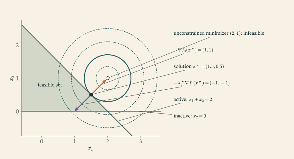
Minimize \(f_0(x)=(x_1-2)^2+(x_2-1)^2\) subject to \(f_1(x)=x_1+x_2-2\le 0\) and \(f_2(x)=-x_2\le 0\) . The problem is convex. Stationarity reads

\[ 2(x_1-2)+\lambda_1=0,\qquad 2(x_2-1)+\lambda_1-\lambda_2=0 . \]

Neither constraint active. Then \(\lambda_1=\lambda_2=0\) and \(x=(2,1)\) . But \(f_1(2,1)=1>0\) : infeasible. Rejected.

Only the first active. Then \(\lambda_2=0\) and \(x_1+x_2=2\) . Stationarity gives \(x_1=2-\lambda_1/2\) and \(x_2=1-\lambda_1/2\) ; substituting, \(3-\lambda_1=2\) , so \(\lambda_1=1\) and \(x=(1.5,0.5)\) . Check what was set aside: \(\lambda_1=1\ge 0\) , and \(f_2=-0.5<0\) . All four conditions hold.

Only the second active. Then \(\lambda_1=0\) , \(x_2=0\) , and stationarity gives \(x_1=2\) and \(\lambda_2=2(0-1)=-2\) . A negative multiplier: rejected.

Both active. Then \(x=(2,0)\) , and stationarity gives \(\lambda_1=0\) from the first equation and \(\lambda_2=-2\) from the second. Rejected for the same reason.

Exactly one case survives: \(x^\star=(1.5,0.5)\) with \(\lambda^\star=(1,0)\) , and by Theorem 6.3 it is the global minimizer, with \(f_0(x^\star)=0.25+0.25=0.5\) . The rejected cases are instructive. A negative multiplier means that the objective could be reduced by moving off the corresponding constraint into the feasible region, so that constraint should not have been treated as active.

6.5 Slater’s condition and strong duality

Theorem 6.3 says that KKT points of convex problems are optimal. It does not say that an optimal point must be a KKT point. By Theorem 6.2, that would follow if strong duality held with the dual optimum attained. So the question becomes: when is the duality gap of a convex problem zero?

The proof that Slater’s condition yields strong duality rests on one geometric theorem about convex sets, which we state without proof. It is a theorem of finite-dimensional convex geometry with no identifier of its own in this library; its counterpart in infinite-dimensional spaces is the Hahn–Banach theorem, treated in Functional Analysis. In \(\mathbb R^k\) it can be proved from the projection theorem of Chapter 9 followed by a limiting argument.

The role of the strictly feasible point is confined to the last paragraph: it excludes a vertical separating hyperplane, one with \(\mu=0\) , which would carry no information about the objective. Two refinements are true and used in practice, though not proved here. Inequality constraints given by affine functions need not hold strictly at the Slater point; and consequently for a problem all of whose constraints are affine, feasibility alone suffices. That is consistent with Theorem 4.10, where strong duality for linear programs needed no interior point.

Combining Theorems 6.2, 6.3, and 6.6 gives the statement that makes convex optimization a closed subject.

The second half of this proof uses Theorem 6.6 in full. For problems with inequality constraints only, everything it uses has been proved above; for problems that also have equality constraints, the corollary rests on the general case of Slater’s theorem, which was stated and not proved.

6.6 Beyond convexity

For a problem that is not convex, Theorem 6.3 is unavailable, and the KKT conditions lose their sufficiency. They remain necessary for local optimality under a regularity assumption on the constraints.

We do not prove this theorem; its proof uses the implicit function theorem to show that every direction tangent to the active constraints is the velocity of a feasible curve, along which the objective cannot decrease to first order. Its hypothesis is the linear independence constraint qualification. Together with Corollary 6.7 it supports a workflow for general problems that parallels Section 3.6: establish that a minimizer exists; check that the qualification holds at every feasible point, or separately examine the points where it fails; find all KKT points; compare objective values.

6.7 Linear and quadratic programs revisited

The results of Chapter 4 are instances of the present theory. For the standard-form linear program, Example 5.2 identified the multipliers: \(y=-\nu\) for the equations and \(\lambda=c-A^{\top}y\) for the sign constraints. The KKT conditions become \(Ax=b\) , \(x\ge 0\) (primal feasibility); \(c-A^{\top}y\ge 0\) (dual feasibility, which is feasibility for the dual program); stationarity, which is the definition of \(\lambda\) ; and \(x_j(c_j-A_j^{\top}y)=0\) (complementary slackness). These are exactly the three ingredients of Theorem 4.11. All constraints are affine, so by the refinement of Slater’s theorem the conditions are necessary and sufficient for optimality whenever the program is feasible and bounded.

For an equality-constrained quadratic program with \(P\succeq 0\) , the conditions are the linear system preceding Theorem 4.13, and Theorem 6.3 reproves part (a) of that theorem. For a convex quadratic program with inequality constraints, the conditions are linear equations together with sign and complementarity conditions, and the active-set enumeration of Example 6.2 is the prototype of the active-set algorithms mentioned in Chapter 10.

With optimality conditions and certificates in hand for both unconstrained and constrained problems, the remaining chapters turn to computation: how to generate a sequence of points that converges to a solution, and how fast.

Exercises

1. Write the KKT conditions for “minimize \(x_1^2+x_2^2\) subject to \(x_1+2x_2\ge 5\) ”, solve them, and confirm the result by computing the dual optimal value.

   Answer

   With \(f_1(x)=5-x_1-2x_2\) : stationarity is \(2x_1-\lambda=0\) , \(2x_2-2\lambda=0\) , so \(x=(\lambda/2,\lambda)\) . The unconstrained minimizer \(0\) is infeasible, so the constraint is active: \(\lambda/2+2\lambda=5\) , giving \(\lambda=2\) and \(x^\star=(1,2)\) with value \(5\) . The dual function is \(g(\lambda)=5\lambda-\tfrac54\lambda^2\) , maximized at \(\lambda=2\) with \(d^\star=5\) .

2. Solve “minimize \((x_1-3)^2+(x_2-2)^2\) subject to \(x_1+x_2\le 4\) and \(x_1\le 2\) ” by enumerating the four active sets, reporting why each rejected case fails; then comment on the multiplier of the first constraint at the solution.

   Solution

   Let \(f_1=x_1+x_2-4\) and \(f_2=x_1-2\) . Stationarity: \(2(x_1-3)+\lambda_1+\lambda_2=0\) and \(2(x_2-2)+\lambda_1=0\) .

   Neither active. \(\lambda=0\) gives \(x=(3,2)\) , where \(f_1=1>0\) . Infeasible; rejected.

   Only \(f_1\) active. \(\lambda_2=0\) , so \(x=(3-\lambda_1/2,\ 2-\lambda_1/2)\) ; the constraint \(x_1+x_2=4\) gives \(\lambda_1=1\) and \(x=(2.5,1.5)\) . But \(f_2=0.5>0\) . Infeasible; rejected.

   Only \(f_2\) active. \(\lambda_1=0\) and \(x_1=2\) . The second stationarity equation gives \(x_2=2\) , and the first gives \(\lambda_2=-2(2-3)=2\ge 0\) . Check the constraint set aside: \(f_1(2,2)=0\le 0\) . Every KKT condition holds, with \(\lambda=(0,2)\) .

   Both active. \(x=(2,2)\) ; the second equation gives \(\lambda_1=0\) and the first gives \(\lambda_2=2\) . The same point and multipliers.

   The problem is convex, so by Theorem 6.3 the solution is \(x^\star=(2,2)\) with \(\lambda^\star=(0,2)\) and optimal value \(1\) . The first constraint is active at the solution, since \(2+2=4\) , and yet its multiplier is zero. Complementary slackness allows this: the product \(\lambda_1f_1\) vanishes because both factors do. The interpretation is that the first constraint is not holding the solution back. If it were deleted, the minimizer over \(x_1\le 2\) alone would still be \((2,2)\) , which merely happens to lie on the line \(x_1+x_2=4\) . By Theorem 5.6, loosening that constraint slightly would not lower the optimal value at all.

3. To maximize \(x_1x_2x_3\) subject to \(x_1+x_2+x_3=3\) and \(x>0\) , first use Proposition 1.7 to replace the objective by one that makes the problem convex, then solve the KKT conditions and justify that the KKT point is the global solution.

   Solution

   On the feasible set all \(x_i\) are positive, so the objective \(x_1x_2x_3\) is positive, and \(\log\) is strictly increasing on \((0,\infty)\) . By Proposition 1.7, maximizing \(x_1x_2x_3\) has the same solutions as maximizing \(\log x_1+\log x_2+\log x_3\) , that is, as minimizing \(f_0(x)=-\sum_i\log x_i\) over the domain \(\mathcal D=\{x>0\}\) subject to \(h(x)=x_1+x_2+x_3-3=0\) .

   This reformulated problem is convex: the Hessian of \(f_0\) is diagonal with entries \(1/x_i^2>0\) , and the constraint is affine. There are no inequality constraints, because positivity is built into the open domain. The KKT conditions are feasibility and stationarity: \(-1/x_i+\nu=0\) for \(i=1,2,3\) . Hence \(x_1=x_2=x_3=1/\nu\) , and the constraint gives \(3/\nu=3\) , so \(\nu=1\) and \(x=(1,1,1)\) .

   By Theorem 6.3 a KKT point of a convex problem is a global minimizer, so \((1,1,1)\) minimizes \(-\sum\log x_i\) and therefore maximizes the product, whose maximal value is \(1\) . In the original form the objective \(-x_1x_2x_3\) is not convex, and the KKT conditions there would only have produced a candidate. The monotone change of objective is what bought the guarantee. As a by-product we have proved \(x_1x_2x_3\le 1\) whenever the \(x_i\) are positive with sum \(3\) , the three-variable inequality between geometric and arithmetic means.

4. Consider a convex problem with differentiable functions for which strong duality holds with the dual optimum attained. Prove that if \((\lambda,\nu)\) are KKT multipliers for one optimal point \(x^\star\) , then they are KKT multipliers for every optimal point.

   Solution

   Let \((\lambda,\nu)\) be KKT multipliers for the optimal point \(x^\star\) . By Theorem 6.3, applied to the KKT triple \((x^\star,\lambda,\nu)\) , the pair \((\lambda,\nu)\) is dual optimal and the duality gap is zero.

   Now let \(x'\) be any other primal optimal point. Then \(x'\) is primal optimal, \((\lambda,\nu)\) is dual optimal, and the gap is zero. These are exactly the hypotheses of Theorem 6.2, which concludes that \((x',\lambda,\nu)\) satisfies the KKT conditions. So the same multipliers serve at every optimal point.

   In fact the argument shows more: the set of KKT multipliers of a convex problem coincides with the set of dual optimal solutions, independently of which primal optimal point is considered. Multipliers are attached to the problem, not to a particular solution. The hypothesis that strong duality holds with the dual attained was not needed separately, since Theorem 6.3 delivers it as soon as one KKT triple exists.

5. For each problem decide whether Slater’s condition holds, whether the optimal point has KKT multipliers, and whether strong duality holds: (a) minimize \(x\) subject to \(x^2\le 0\) ; (b) minimize \(x_1\) subject to \(x_1^2+x_2^2\le 1\) and \((x_1-2)^2+x_2^2\le 1\) ; (c) minimize \(x^2\) subject to \(x\ge 1\) .

   Solution

   (a) Slater fails, since no \(x\) satisfies \(x^2<0\) . Example 6.5 shows that the optimal point \(x=0\) has no multipliers, and that \(d^\star=p^\star=0\) with the dual supremum not attained. So strong duality holds as an equality of values, without a dual optimal point.

   (b) The first disc is centred at the origin and the second at \((2,0)\) , both of radius \(1\) ; they meet only at \((1,0)\) . The feasible set is that single point, so Slater fails: no point is strictly inside both discs. The optimal point is \((1,0)\) with \(p^\star=1\) . The gradients there are \(\nabla f_0=(1,0)\) , \(\nabla f_1=(2,0)\) , \(\nabla f_2=(2(1-2),0)=(-2,0)\) , and stationarity \(1+2\lambda_1-2\lambda_2=0\) is solved, for example, by \(\lambda=(0,\tfrac12)\) . Both constraints are active, so complementary slackness holds. Multipliers exist, and by Theorem 6.3 strong duality holds with the dual optimum attained.

   (c) Slater holds: \(x=2\) gives \(1-x=-1<0\) . By Corollary 6.7 the optimal point \(x=1\) has a multiplier, namely \(\lambda=2\) , and strong duality holds (Example 5.1).

   The three cases show that Slater’s condition is sufficient for the existence of multipliers and not necessary: it fails in both (a) and (b), and multipliers are absent in (a) but present in (b).

6. A student solving “minimize \((x_1-1)^2+(x_2-1)^2\) subject to \(x_1+x_2\le 4\) ” writes complementary slackness as “\(\lambda=0\) and \(x_1+x_2=4\) ”, obtains \(x=(1,1)\) from stationarity, notes that \(1+1\ne 4\) , and declares that the problem has no solution. Diagnose the error and solve the problem correctly.

   Solution

   The error is in complementary slackness. The condition is \(\lambda(x_1+x_2-4)=0\) , a product, which is satisfied if either factor vanishes. The student imposed both \(\lambda=0\) and \(x_1+x_2=4\) , which is one very special situation and not what the condition says. Having over-constrained the system, the student found it inconsistent and blamed the problem.

   Done correctly, there are two cases. If \(\lambda=0\) , stationarity \(2(x_1-1)+\lambda=0\) , \(2(x_2-1)+\lambda=0\) gives \(x=(1,1)\) , and primal feasibility holds because \(1+1=2\le 4\) ; dual feasibility holds because \(\lambda=0\ge 0\) . All four conditions are satisfied. If instead the constraint is active, stationarity gives \(x_1=x_2=1-\lambda/2\) and \(x_1+x_2=4\) gives \(\lambda=-2\) , which violates dual feasibility; this case is rejected.

   The problem is convex, so by Theorem 6.3 the solution is \(x^\star=(1,1)\) with \(\lambda^\star=0\) and optimal value \(0\) . The constraint is inactive: the unconstrained minimizer was feasible all along, and the constraint could have been ignored. A problem with a continuous coercive objective and a nonempty closed feasible set always has a solution, so a conclusion of “no solution” should itself have been a warning.

7. In Example 6.4 the bound \(x_1\le 1\) has multiplier \(6\) . Predict the optimal value when the bound becomes \(x_1\le 1.1\) , compute the exact new optimal value, and say which of the two numbers Theorem 5.6 guarantees to be the smaller.

   Solution

   Theorem 5.6 gives \(p^\star(u)\ge p^\star(0)-\lambda^\star u\) , and for small \(u\) the right side is also the first-order prediction. With \(p^\star(0)=9\) , \(\lambda^\star=6\) , and \(u=0.1\) , the predicted value is \(9-0.6=8.4\) .

   Exactly: with the bound \(x_1\le 1.1\) still active, \(x=(1.1,\ 1.9)\) and the value is \(1.21+2\cdot 3.61=8.43\) . To confirm that this is optimal, check the KKT conditions: \(4x_2+\nu=0\) gives \(\nu=-7.6\) , and \(2x_1+\lambda+\nu=0\) gives \(\lambda=5.4\ge 0\) .

   The theorem guarantees that the prediction is the smaller number: \(8.4\le 8.43\) . The difference \(0.03\) is the second-order term \(3u^2\) found in Example 6.4. The multiplier has dropped from \(6\) to \(5.4\) , reflecting that each further relaxation is worth a little less; the constraint stops being active altogether when the bound reaches \(x_1=2\) .

8. Find all KKT points of “minimize \(x_1x_2\) subject to \(x_1^2+x_2^2\le 2\) ”, evaluate the objective at each, and identify the global minimizers, explaining why a global minimizer exists and must be among the KKT points.

   Solution

   With \(f_1=x_1^2+x_2^2-2\) , the conditions are \(x_2+2\lambda x_1=0\) , \(x_1+2\lambda x_2=0\) , \(\lambda\ge 0\) , \(\lambda f_1=0\) , \(f_1\le 0\) .

   If \(\lambda=0\) : \(x=(0,0)\) , feasible, with objective \(0\) . If \(\lambda>0\) the constraint is active. Substituting \(x_2=-2\lambda x_1\) into the second equation gives \(x_1(1-4\lambda^2)=0\) . If \(x_1=0\) then \(x_2=0\) , which is not on the circle; so \(\lambda=\tfrac12\) , \(x_2=-x_1\) , and \(2x_1^2=2\) gives the points \((1,-1)\) and \((-1,1)\) , each with objective \(-1\) . The points \((1,1)\) and \((-1,-1)\) would need \(\lambda=-\tfrac12\) and are not KKT points.

   So there are three KKT points: \((0,0)\) with \(\lambda=0\) and value \(0\) , and \((1,-1)\) , \((-1,1)\) with \(\lambda=\tfrac12\) and value \(-1\) .

   A global minimizer exists by Theorem 1.4, because the disc is compact and the objective continuous. It must be a KKT point by Theorem 6.8: at interior points no constraint is active, and on the circle the single active gradient \((2x_1,2x_2)\) is nonzero, so the linear independence qualification holds everywhere. Comparing values, the global minimizers are \((1,-1)\) and \((-1,1)\) with \(p^\star=-1\) . The origin is a KKT point that is not a local minimizer: it is the saddle of \(x_1x_2\) . The objective is not convex, so Theorem 6.3 did not apply, and the comparison step was necessary.

9. Project the point \(a=(0.4,\ 0.9,\ -0.2,\ 0.5)\) onto the probability simplex in \(\mathbb R^4\) using the formula \(x_i=\max\{a_i-\nu,0\}\) of Example 6.3, reporting \(\nu\) and the multipliers of the sign constraints.

   Answer

   With all four coordinates positive, \(1.6-4\nu=1\) gives \(\nu=0.15\) , but then \(a_3-\nu<0\) . With the three largest, \(1.8-3\nu=1\) gives \(\nu=4/15\approx 0.267\) , consistent. So \(x^\star=(2/15,\ 19/30,\ 0,\ 7/30)\approx(0.133,\ 0.633,\ 0,\ 0.233)\) , with multipliers \(\lambda^\star=(0,0,\nu-a_3,0)=(0,0,7/15,0)\) .

10. Write out the KKT conditions for the standard-form linear program directly from Definition 6.1 and show that, after eliminating the multipliers of the sign constraints, they are primal feasibility, dual feasibility in the sense of Definition 4.8, and the complementary slackness of Theorem 4.11.

    Hint

    With multipliers \(\lambda\ge 0\) for \(-x\le 0\) and \(\nu\) for \(Ax-b=0\) , stationarity is \(c-\lambda+A^{\top}\nu=0\) . Put \(y=-\nu\) and eliminate \(\lambda=c-A^{\top}y\) ; then \(\lambda\ge 0\) is \(A^{\top}y\le c\) and \(\lambda_jx_j=0\) is the condition of Theorem 4.11.

11. The problem “minimize \(x_1+x_2\) subject to \(x_1x_2\ge 1\) , \(x>0\) ” has a convex feasible set (Example 2.1), but the constraint function \(1-x_1x_2\) is not convex. Find the KKT point, then rewrite the constraint with a convex function so that Theorem 6.3 applies, and conclude.

    Solution

    With \(f_1(x)=1-x_1x_2\) and multiplier \(\lambda\) , stationarity is \(1-\lambda x_2=0\) and \(1-\lambda x_1=0\) . These force \(\lambda\ne 0\) , so the constraint is active, and \(x_1=x_2=1/\lambda\) . Then \(x_1x_2=1\) gives \(\lambda^2=1\) , and positivity of \(x\) selects \(\lambda=1\) , \(x=(1,1)\) , with objective \(2\) . Since \(f_1\) is not convex (its Hessian has eigenvalues \(\pm1\) ), Theorem 6.3 does not apply to this formulation, and so far \((1,1)\) is only a candidate.

    On the domain \(x>0\) the logarithm is strictly increasing, so \(x_1x_2\ge 1\) is equivalent to \(\log x_1+\log x_2\ge 0\) , that is, to \(\tilde f_1(x)=-\log x_1-\log x_2\le 0\) . The function \(\tilde f_1\) is convex, with diagonal Hessian entries \(1/x_i^2\) . The feasible set is unchanged, the objective is linear, and the problem is now convex in the sense required by Theorem 6.3. Its KKT conditions, with multiplier \(\mu\) , are \(1-\mu/x_1=0\) , \(1-\mu/x_2=0\) , so \(x_1=x_2=\mu>0\) and the constraint is active: \(-2\log\mu=0\) , giving \(\mu=1\) and \(x=(1,1)\) .

    Theorem 6.3 now certifies that \((1,1)\) is the global minimizer, with \(p^\star=2\) . The feasible set was convex all along; what the first formulation lacked was a convex description of it. The same set can be described by convex or nonconvex constraint functions, and the theorems apply to descriptions.

12. For “minimize \(x\) subject to \(x\ge 0\) and \(x\le 0\) ” show that no strictly feasible point exists, that KKT multipliers nevertheless exist, and say which refinement of Slater’s theorem explains this.

    Answer

    Strict feasibility would need \(x>0\) and \(x<0\) together. With \(f_1=-x\) and \(f_2=x\) , stationarity at \(x=0\) is \(1-\lambda_1+\lambda_2=0\) , solved by \(\lambda=(1,0)\) , and both constraints are active. The refinement that affine inequality constraints need not hold strictly explains it: all constraints here are affine, so feasibility suffices.

13. The set \(\{x\in\mathbb R^2:x_1^2+x_2^2\le 2,\ x_2\le 1\}\) has a corner at \((1,1)\) where both constraints are active. Describe all cost vectors \(c\) for which \((1,1)\) minimizes \(c^{\top}x\) over the set, and test your description on \(c=(-1,-3)\) and \(c=(-3,-1)\) .

    Solution

    The problem of minimizing \(c^{\top}x\) over the set is convex, and Slater’s condition holds, for instance at the origin. By Corollary 6.7, \((1,1)\) is optimal if and only if multipliers \(\lambda_1,\lambda_2\ge 0\) exist with

    \[ c+\lambda_1\begin{pmatrix}2\\2\end{pmatrix}+\lambda_2\begin{pmatrix}0\\1\end{pmatrix}=0, \]

    where \((2,2)\) and \((0,1)\) are the gradients of \(x_1^2+x_2^2-2\) and \(x_2-1\) at \((1,1)\) ; complementary slackness is automatic because both constraints are active. So \((1,1)\) is optimal exactly when \(-c\) lies in the cone generated by \((1,1)\) and \((0,1)\) . Solving, \(\lambda_1=-c_1/2\) and \(\lambda_2=c_1-c_2\) , so the condition is \(c_1\le 0\) and \(c_2\le c_1\) .

    For \(c=(-1,-3)\) : \(\lambda_1=\tfrac12\) and \(\lambda_2=-1+3=2\) , both nonnegative, so \((1,1)\) is optimal, with value \(-4\) . For \(c=(-3,-1)\) : \(\lambda_1=\tfrac32\) and \(\lambda_2=-3+1=-2<0\) , so \((1,1)\) is not optimal. Indeed the point \(\sqrt2\,(3,1)/\sqrt{10}\approx(1.342,\ 0.447)\) on the circle is feasible and has value \(-\sqrt{20}\approx-4.472\) , below the value \(-4\) at \((1,1)\) . The negative multiplier on \(x_2\le 1\) says that the objective improves by moving off that constraint, down along the circle.

14. For a convex problem satisfying Slater’s condition, prove that if the \(i\) -th inequality constraint is inactive at some optimal point, then \(\lambda_i^\star=0\) for every dual optimal \(\lambda^\star\) .

    Hint

    By Theorem 6.6 strong duality holds and the dual is attained. Apply Theorem 6.2 to the given optimal point paired with an arbitrary dual optimal \(\lambda^\star\) : complementary slackness gives \(\lambda_i^\star f_i(x^\star)=0\) with \(f_i(x^\star)<0\) . If the problem has equality constraints, this argument uses the general case of Theorem 6.6, which the manual states without proof.

15. Show that with no constraints Theorem 6.3 reduces to the sufficiency half of Theorem 3.5, and that with a quadratic objective and constraints \(Ax=b\) only, the KKT conditions are the linear system preceding Theorem 4.13.

    Hint

    With \(m=p=0\) the conditions are just \(\nabla f_0(x)=0\) , and the Lagrangian is \(f_0\) . With \(f_0=\tfrac12x^{\top}Px+q^{\top}x\) and \(h(x)=Ax-b\) , stationarity is \(Px+q+A^{\top}\nu=0\) and feasibility is \(Ax=b\) .

16. Consider “minimize \(x_1\) subject to \(x_2-x_1^3\le 0\) and \(-x_2\le 0\) ”. Show that \((0,0)\) is the global minimizer, that no KKT multipliers exist there, and identify which hypothesis of Theorem 6.8 fails.

    Solution

    Feasibility requires \(0\le x_2\le x_1^3\) , which forces \(x_1^3\ge 0\) , that is, \(x_1\ge 0\) . So the objective \(x_1\) is at least \(0\) on the feasible set, and \((0,0)\) is feasible with value \(0\) . It is the global minimizer; it is in fact the only feasible point with \(x_1=0\) .

    At the origin both constraints are active. Their gradients are \(\nabla f_1=(-3x_1^2,\,1)=(0,1)\) and \(\nabla f_2=(0,-1)\) , and \(\nabla f_0=(1,0)\) . Stationarity would require

    \[ \begin{pmatrix}1\\0\end{pmatrix}+\lambda_1\begin{pmatrix}0\\1\end{pmatrix}+\lambda_2\begin{pmatrix}0\\-1\end{pmatrix}=\begin{pmatrix}0\\0\end{pmatrix}, \]

    whose first component reads \(1=0\) . No multipliers exist.

    Theorem 6.8 requires the active constraint gradients to be linearly independent, and here \((0,1)\) and \((0,-1)\) are parallel. Geometrically the feasible set has a cusp at the origin: the two boundary curves \(x_2=x_1^3\) and \(x_2=0\) are tangent there, and the constraint gradients, both vertical, cannot produce the horizontal direction needed to balance the objective. Corollary 6.7 does not apply either, since \(x_2-x_1^3\) is not a convex function. The example shows that a minimizer can fail to be a KKT point, so a search restricted to KKT points must be accompanied by a check of the qualification.

17. For Example 6.2 compute the dual function \(g(\lambda_1,\lambda_2)\) in closed form, evaluate it at \(\lambda=(1,0)\) , and confirm that it equals the primal optimal value.

    Answer

    Minimizing the Lagrangian gives \(x_1=2-\lambda_1/2\) and \(x_2=1-(\lambda_1-\lambda_2)/2\) , and \(g(\lambda)=\lambda_1-\lambda_2-\tfrac14\lambda_1^2-\tfrac14(\lambda_1-\lambda_2)^2\) . At \(\lambda=(1,0)\) : \(g=1-\tfrac14-\tfrac14=\tfrac12\) , equal to the primal optimal value \(0.5\) .

18. For “minimize \(x^2\) subject to \(x\le 0\) ” find the KKT point and its multiplier, note that the constraint is active with zero multiplier, and compute the perturbation function \(p^\star(u)\) for the constraint \(x\le u\) to see what a zero multiplier means for sensitivity.

    Answer

    The KKT point is \(x=0\) with \(\lambda=0\) : stationarity \(2x+\lambda=0\) and the constraint active. The perturbation function is \(p^\star(u)=0\) for \(u\ge 0\) and \(u^2\) for \(u<0\) . Its derivative at \(0\) is \(0=-\lambda\) : to first order, neither tightening nor loosening the constraint changes the optimal value.

19. For the problem of Example 6.2, examine the candidate points \((2,0)\) , \((1,1)\) , and \((1.5,0.5)\) : for each, list the active constraints, solve stationarity for the multipliers if possible, and state which KKT condition, if any, fails.

    Answer

    \((2,0)\) : both constraints active; stationarity gives \(\lambda_1=0\) , \(\lambda_2=-2\) ; dual feasibility fails. \((1,1)\) : only \(f_1\) active, so \(\lambda_2=0\) ; the two stationarity equations give \(\lambda_1=2\) and \(\lambda_1=0\) , which is inconsistent; stationarity fails. \((1.5,0.5)\) : only \(f_1\) active; \(\lambda=(1,0)\) ; all conditions hold.

20. Solve “minimize \(\tfrac12(x_1^2+x_2^2)-x_1-3x_2\) subject to \(x_1+x_2\le 1\) , \(x_1\ge 0\) , \(x_2\ge 0\) ” with the KKT conditions, starting from the guess that only the first constraint is active and revising the guess when it fails.

    Solution

    Write the constraints as \(f_1=x_1+x_2-1\le 0\) , \(f_2=-x_1\le 0\) , \(f_3=-x_2\le 0\) with multipliers \(\lambda,\mu_1,\mu_2\) . Stationarity:

    \[ x_1-1+\lambda-\mu_1=0,\qquad x_2-3+\lambda-\mu_2=0 . \]

    The unconstrained minimizer \((1,3)\) violates \(f_1\) , so some constraint is active.

    Guess: only \(f_1\) active. Then \(\mu=0\) , \(x=(1-\lambda,\ 3-\lambda)\) , and \(x_1+x_2=1\) gives \(\lambda=1.5\) , \(x=(-0.5,\ 1.5)\) . This violates \(x_1\ge 0\) . The guess fails, and the way it fails suggests the repair: the sign constraint on \(x_1\) should be active as well.

    Revised guess: \(f_1\) and \(f_2\) active. Then \(x_1=0\) , \(x_2=1\) , and \(\mu_2=0\) . The second stationarity equation gives \(\lambda=3-1=2\) , and the first gives \(\mu_1=x_1-1+\lambda=1\) . Both multipliers are nonnegative, and the remaining constraint holds strictly, \(x_2=1>0\) , consistent with \(\mu_2=0\) .

    All KKT conditions hold at \(x^\star=(0,1)\) with \(\lambda^\star=2\) , \(\mu^\star=(1,0)\) . The objective is convex (its Hessian is the identity) and the constraints are affine, so by Theorem 6.3 this is the global minimizer. The optimal value is \(\tfrac12(0+1)-0-3=-2.5\) .