An algorithm working on a constrained problem reports a feasible point with objective value \(2.44\) . Is that good? The question cannot be answered by looking at feasible points, because every feasible point only shows that the optimal value is at most something. To know how far \(2.44\) is from optimal one needs a number on the other side: a guaranteed lower bound on what any feasible point can achieve.
Chapter 4 produced such bounds for linear programs, from a dual program whose every feasible point bounds the primal. This chapter shows that the construction owes nothing to linearity. Attach a price to each constraint, let the prices pay for violations, and minimize the resulting unconstrained function: whatever value comes out is a lower bound on the constrained optimum. The bound exists for every problem, convex or not. Whether the best such bound actually equals the optimal value is a separate and deeper question, settled for convex problems in Chapter 6.
5.1 Pricing the constraints
Take the standard-form problem of Definition 1.1 with domain \(\mathcal D\) , optimal value \(p^\star\) , and no assumption of convexity:
Definition 5.1 (Lagrangian). The Lagrangian of the problem is the function \(L:\mathcal D\times\mathbb R^m\times\mathbb R^p\to\mathbb R\) ,
The numbers \(\lambda_i\) and \(\nu_j\) are the Lagrange multipliers, or dual variables, associated with the constraints \(f_i(x)\le 0\) and \(h_j(x)=0\) .
Read \(\lambda_i\) as a price per unit of the quantity \(f_i(x)\) . If \(\lambda_i\ge 0\) , a violation \(f_i(x)>0\) is charged, and slack \(f_i(x)<0\) earns a rebate. The hard requirement \(f_i(x)\le 0\) has been replaced by a linear charge. The replacement is generous to the minimizer in one precise sense: at a feasible point every charge is nonpositive when \(\lambda\ge 0\) , and the equality terms vanish, so
That single inequality is the engine of the whole chapter. It depends on two conventions that must be kept fixed: inequality constraints are written with \(\le 0\) , and their multipliers are nonnegative. Equality multipliers may have either sign, because \(h_j(x)\) is zero at feasible points regardless.
Definition 5.2 (dual function). The Lagrange dual function \(g:\mathbb R^m\times\mathbb R^p\to[-\infty,\infty)\) is
The infimum is over the whole domain, not over the feasible set: the constraints have been priced, not imposed. It may equal \(-\infty\) for some multipliers, and that is allowed.
Proposition 5.3 (the dual function is concave). For any problem whatever, \(g\) is a concave function of \((\lambda,\nu)\) .
Proof. For each fixed \(x\in\mathcal D\) , the function \((\lambda,\nu)\mapsto L(x,\lambda,\nu)\) is affine. Hence \(-L(x,\cdot,\cdot)\) is affine, in particular convex, and \(-g=\sup_{x\in\mathcal D}\bigl(-L(x,\cdot,\cdot)\bigr)\) is a pointwise supremum of convex functions. By Proposition 2.7(c), in the form extended to arbitrary families, \(-g\) is convex wherever it is finite, and the defining inequality holds trivially where it is \(+\infty\) .
The concavity of \(g\) is free. It does not depend on \(f_0\) or the constraints being convex, and it means that maximizing \(g\) is always a convex optimization problem, even when the original problem is not.
5.2 Every dual value is a lower bound
Theorem 5.4 (lower bound property). For every \(\lambda\ge 0\) and every \(\nu\) ,
Proof. If the problem is infeasible, \(p^\star=+\infty\) and there is nothing to prove. Otherwise let \(\tilde x\) be any feasible point. Then \(\lambda_if_i(\tilde x)\le 0\) for each \(i\) and \(\nu_jh_j(\tilde x)=0\) for each \(j\) , so \(L(\tilde x,\lambda,\nu)\le f_0(\tilde x)\) . Therefore
Since this holds for every feasible \(\tilde x\) , taking the infimum over feasible points gives \(g(\lambda,\nu)\le p^\star\) .
The proof is three lines and uses nothing but signs. It is worth being able to reproduce on demand, because each of its steps corresponds to a way the bound can be broken: by a negative \(\lambda_i\) , by a constraint written in the wrong direction, or by minimizing the Lagrangian over less than the whole domain.
Definition 5.5 (dual problem, duality gap). The Lagrange dual problem is
Its optimal value is denoted \(d^\star\) . A pair \((\lambda,\nu)\) with \(\lambda\ge 0\) and \(g(\lambda,\nu)>-\infty\) is dual feasible. The inequality \(d^\star\le p^\star\) , which follows from Theorem 5.4, is weak duality; the nonnegative number \(p^\star-d^\star\) is the duality gap; and strong duality means \(d^\star=p^\star\) . The original problem is called the primal.
Example 5.1: A scalar dual computed in full
Minimize \(x^2\) subject to \(x\ge 1\) . In standard form the constraint is \(f_1(x)=1-x\le 0\) . The primal solution is evidently \(x^\star=1\) with \(p^\star=1\) ; the point of the example is to see the dual machinery reproduce it.
The Lagrangian is \(L(x,\lambda)=x^2+\lambda(1-x)\) . For fixed \(\lambda\) it is a convex quadratic in \(x\) , minimized where \(2x-\lambda=0\) , that is, at \(x=\lambda/2\) . Substituting,
Each value is a lower bound on \(p^\star\) : \(g(0)=0\) , \(g(1)=0.75\) , \(g(3)=0.75\) . The best bound maximizes the concave function \(g\) over \(\lambda\ge 0\) : \(g'(\lambda)=1-\lambda/2=0\) at \(\lambda^\star=2\) , where \(g(2)=2-1=1\) . So \(d^\star=1=p^\star\) and strong duality holds. Moreover the minimizer of the Lagrangian at the optimal price, \(x=\lambda^\star/2=1\) , is the primal solution.
The left panel of Figure 5.1 below plots this dual function. Every point on the curve lies on or below the dashed line at height \(p^\star\) , as Theorem 5.4 demands, and the curve touches the line at one price.
5.3 Duals of familiar problems
The usefulness of the dual depends on being able to compute \(g\) . For linear and quadratic problems the inner minimization can be done in closed form.
Example 5.2: The linear programming dual, derived
Take the standard-form linear program of Definition 4.1: minimize \(c^{\top}x\) subject to \(Ax=b\) and \(x\ge 0\) . Write the sign constraints as \(-x_i\le 0\) with multipliers \(\lambda_i\ge 0\) , and the equations as \(Ax-b=0\) with multipliers \(\nu\) . Then
This is affine in \(x\) . An affine function on \(\mathbb R^n\) is unbounded below unless its linear part vanishes, so
The dual problem maximizes \(-b^{\top}\nu\) subject to \(\lambda=c+A^{\top}\nu\) and \(\lambda\ge 0\) . Eliminating \(\lambda\) leaves the constraint \(c+A^{\top}\nu\ge 0\) . With \(y=-\nu\) this is: maximize \(b^{\top}y\) subject to \(A^{\top}y\le c\) . That is exactly the dual of Definition 4.8, which there was written down by fiat.
The eliminated multiplier has a meaning too: \(\lambda=c-A^{\top}y\) is the vector of reduced costs. For the workshop problem, \(y=(-1,-1)\) gives \(\lambda=(-3,-2,0,0)+(3,2,1,1)=(0,0,1,1)\) , the reduced costs found in the third pass of Example 4.3, and \(g=b^{\top}y=-9=p^\star\) .
Example 5.3: A least-norm problem
Minimize \(x^{\top}x\) subject to \(Ax=b\) , where \(A\) is \(p\times n\) with independent rows. There are no inequality constraints. The Lagrangian \(L(x,\nu)=x^{\top}x+\nu^{\top}(Ax-b)\) is a strictly convex quadratic in \(x\) with gradient \(2x+A^{\top}\nu\) , minimized at \(x=-\tfrac12A^{\top}\nu\) . Substituting,
The dual problem is the unconstrained maximization of this concave quadratic over \(\nu\in\mathbb R^p\) . Its solution is \(\nu^\star=-2(AA^{\top})^{-1}b\) , and the corresponding \(x=-\tfrac12A^{\top}\nu^\star=A^{\top}(AA^{\top})^{-1}b\) is the least-norm solution of \(Ax=b\) .
With numbers: let \(A=\begin{pmatrix}1&2\end{pmatrix}\) and \(b=5\) . Then \(AA^{\top}=5\) and \(g(\nu)=-\tfrac54\nu^2-5\nu\) , maximized at \(\nu^\star=-2\) with \(d^\star=-5+10=5\) . The corresponding point is \(x=-\tfrac12A^{\top}\nu^\star=(1,2)\) , which is feasible since \(1+4=5\) , and its objective value is \(1+4=5\) . Primal value and dual value agree, so by weak duality \(x=(1,2)\) is optimal: a certificate obtained without any separate optimality argument for the primal. The primal has two variables and the dual has one; when there are many variables and few constraints, the dual is the smaller problem.
5.4 When the bound is not tight
For the convex problems above the best dual bound equalled the primal optimal value. Nothing in Theorem 5.4 promises that.
Example 5.4: A duality gap, and a formulation that removes it
Minimize \(f_0(x)=-x^2\) subject to \(x\le 1\) , with domain \(\mathcal D=[0,2]\) . The objective is concave, so this is not a convex problem. The feasible set is \([0,1]\) , and the minimum of \(-x^2\) there is at \(x=1\) : \(p^\star=-1\) .
The Lagrangian \(L(x,\lambda)=-x^2+\lambda(x-1)\) is a concave function of \(x\) , so its minimum over the interval \([0,2]\) is attained at an endpoint. At \(x=0\) it equals \(-\lambda\) and at \(x=2\) it equals \(-4+\lambda\) . Hence
This is a concave piecewise linear function, increasing for \(\lambda<2\) and decreasing for \(\lambda>2\) , so \(d^\star=g(2)=-2\) . The duality gap is \(p^\star-d^\star=-1-(-2)=1\) . No choice of price brings the bound up to the true optimal value. Notice what happens at \(\lambda=2\) : the Lagrangian is minimized at both endpoints \(x=0\) and \(x=2\) , of which the first is feasible but far from optimal and the second is infeasible. No minimizer of the Lagrangian is the primal solution \(x=1\) .
The dual depends on how the problem is written, not only on its feasible set and objective. Consider minimizing \(-x^2\) over the interval \(-1\le x\le 1\) , with \(\mathcal D=\mathbb R\) , where \(p^\star=-1\) . Written with two affine constraints \(x-1\le 0\) and \(-x-1\le 0\) , the Lagrangian \(-x^2+\lambda_1(x-1)+\lambda_2(-x-1)\) is unbounded below in \(x\) for every choice of prices, so \(g\equiv-\infty\) , \(d^\star=-\infty\) , and the gap is infinite. Written with the single constraint \(x^2-1\le 0\) , the Lagrangian is \((\lambda-1)x^2-\lambda\) , whose infimum over \(x\) is \(-\lambda\) when \(\lambda\ge 1\) and \(-\infty\) otherwise. Then \(d^\star=g(1)=-1=p^\star\) : no gap. Same feasible set, same objective, different duals.
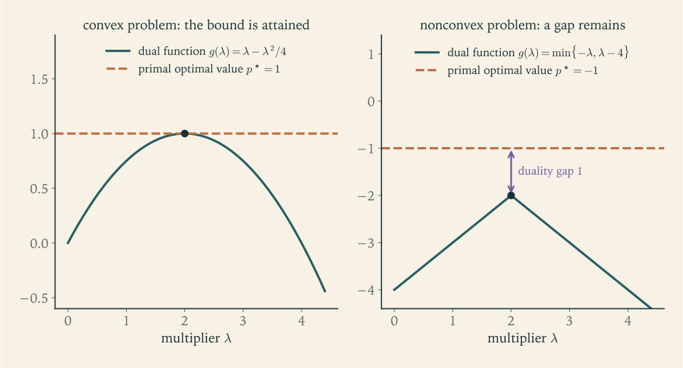
Figure 5.1 separates what is always true from what requires hypotheses. Concavity of \(g\) and the inequality \(g\le p^\star\) appear in both panels. Contact between the curve and the dashed line appears only on the left.
Weak duality can also be read as a statement about the order of two operations. For a fixed \(x\in\mathcal D\) , consider the supremum of \(L(x,\lambda,\nu)\) over \(\lambda\ge 0\) and all \(\nu\) . If \(x\) is feasible, the best the prices can do is to make every charge zero, and the supremum is \(f_0(x)\) . If \(x\) violates a constraint, the corresponding price can be sent to infinity with the appropriate sign, and the supremum is \(+\infty\) . So
The primal and dual optimal values are the same expression with the infimum and the supremum interchanged, and weak duality is the general fact that a supremum of infima never exceeds the corresponding infimum of suprema (Exercise 6). In the language of games, the player who commits first is at a disadvantage; strong duality says that for this particular game the order does not matter.
5.5 Multipliers as sensitivities
Shadow prices in linear programming measured the value of relaxing a constraint. The same interpretation holds in general, as a global inequality. Perturb the problem by allowing each constraint to be violated, or tightened, by a prescribed amount:
and let \(p^\star(u,v)\) be its optimal value, so that \(p^\star(0,0)=p^\star\) . Increasing \(u_i\) enlarges the feasible set, so \(p^\star\) is nonincreasing in each \(u_i\) by Proposition 1.8.
Theorem 5.6 (global sensitivity inequality). Suppose strong duality holds for the unperturbed problem and the dual optimum is attained at \((\lambda^\star,\nu^\star)\) . Then for all \(u\in\mathbb R^m\) and \(v\in\mathbb R^p\) ,
Proof. Let \(x\) be feasible for the perturbed problem. By strong duality and the definition of \(g\) ,
where the last step uses \(f_i(x)\le u_i\) , \(\lambda_i^\star\ge 0\) , and \(h_j(x)=v_j\) . Rearranging, \(f_0(x)\ge p^\star(0,0)-\lambda^{\star\top}u-\nu^{\star\top}v\) for every \(x\) feasible for the perturbed problem; take the infimum over such \(x\) .
The inequality has an asymmetric reading. If \(\lambda_i^\star\) is large and the \(i\) -th constraint is tightened (\(u_i<0\) ), the optimal value is guaranteed to rise by at least \(\lambda_i^\star\lvert u_i\rvert\) : the constraint is expensive. If \(\lambda_i^\star\) is small and the constraint is loosened (\(u_i>0\) ), the optimal value cannot fall by more than \(\lambda_i^\star u_i\) : there is little to gain. The theorem gives no guarantee in the other two directions; loosening an expensive constraint might help a lot or hardly at all. When \(p^\star(u,v)\) happens to be differentiable at the origin, the inequality forces \(\partial p^\star/\partial u_i=-\lambda_i^\star\) there, so the multiplier is exactly the local rate of improvement per unit of relaxation.
Example 5.5: The perturbation function of a scalar problem
Perturb Example 5.1: minimize \(x^2\) subject to \(1-x\le u\) , that is, \(x\ge 1-u\) . If \(u\le 1\) the nearest feasible point to the unconstrained minimizer \(0\) is \(x=1-u\) , so \(p^\star(u)=(1-u)^2\) . If \(u\ge 1\) the point \(x=0\) is feasible and \(p^\star(u)=0\) .
Theorem 5.6 with \(\lambda^\star=2\) asserts \(p^\star(u)\ge 1-2u\) for all \(u\) . For \(u\le 1\) this is \((1-u)^2-(1-2u)=u^2\ge 0\) , and for \(u>1\) the right side is negative. The bound is the tangent line to the convex function \(p^\star\) at \(u=0\) , where the slope is \(\tfrac{d}{du}(1-u)^2=-2=-\lambda^\star\) . Tightening the constraint to \(x\ge 2\) , which is \(u=-1\) , raises the optimal value from \(1\) to \(4\) ; the theorem guaranteed at least \(1+2=3\) .
5.6 Dual values as stopping criteria
Return to the question that opened the chapter.
Proposition 5.7 (certified suboptimality). Let \(x\) be primal feasible and \((\lambda,\nu)\) dual feasible. Then
and likewise \(d^\star-g(\lambda,\nu)\le f_0(x)-g(\lambda,\nu)\) . In particular, if \(f_0(x)=g(\lambda,\nu)\) then \(x\) is primal optimal, \((\lambda,\nu)\) is dual optimal, and strong duality holds.
Proof. By Theorem 5.4 and feasibility of \(x\) , \(g(\lambda,\nu)\le d^\star\le p^\star\le f_0(x)\) . Both claims are rearrangements of this chain, and if its two ends are equal all four numbers coincide.
The quantity \(f_0(x)-g(\lambda,\nu)\) is the duality gap of the pair. It is computable from quantities the algorithm has in hand, and it bounds the unknown error \(f_0(x)-p^\star\) . An algorithm that maintains a feasible \(x\) and a dual feasible \((\lambda,\nu)\) can therefore stop with a guarantee: when the gap of the pair falls below a tolerance \(\varepsilon\) , the point \(x\) is within \(\varepsilon\) of optimal, whether or not the algorithm has converged in any other sense. The pair plays the role, for a general problem, of the primal–dual certificate of Section 4.5.
Example 5.6: Bounding the error before the algorithm finishes
Minimize \(x_1^2+x_2^2\) subject to \(x_1+x_2\ge 2\) . In standard form \(f_1(x)=2-x_1-x_2\le 0\) . The Lagrangian \(x_1^2+x_2^2+\lambda(2-x_1-x_2)\) separates into two copies of \(x_i^2-\lambda x_i\) , each minimized at \(x_i=\lambda/2\) with value \(-\lambda^2/4\) , so
Suppose an algorithm has reached the feasible point \(x=(1.2,1.0)\) , with \(f_0(x)=1.44+1=2.44\) , and holds the price estimate \(\lambda=1.8\) . Then \(g(1.8)=3.6-1.62=1.98\) . Without knowing the solution we can assert
so the current point is within \(0.46\) of optimal. The true values are \(x^\star=(1,1)\) , \(p^\star=2\) , and \(\lambda^\star=2\) , with \(g(2)=4-2=2\) ; the actual error of the point is \(0.44\) , inside the certified bound. A better price estimate would tighten the lower bound, and a better point the upper bound; the two are improved independently.
Common mistake. Giving an inequality multiplier the wrong sign, or reversing a constraint without reversing the sign. Suppose the constraint \(x\ge 1\) of Example 5.1 is carelessly written as \(x-1\le 0\) . The Lagrangian becomes \(x^2+\lambda(x-1)\) and the dual function \(-\lambda-\lambda^2/4\) , whose maximum over \(\lambda\ge 0\) is \(0\) at \(\lambda=0\) . That is a correct statement about a different problem, minimize \(x^2\) subject to \(x\le 1\) , whose optimal value is indeed \(0\) . Applied to the intended problem it would suggest a duality gap of \(1\) where there is none. To repair such an error, normalise every inequality to the form \(f_i(x)\le 0\) , require \(\lambda_i\ge 0\) , and rederive the lower bound of Theorem 5.4 line by line for the problem as written. If a term \(\lambda_if_i(\tilde x)\) is not visibly nonpositive at feasible points, a sign is wrong.
Weak duality asks nothing of the problem. Strong duality asks a great deal, and when it holds it does more than certify values: it ties the primal and dual solutions together through a system of equations and inequalities. Deriving that system, the Karush–Kuhn–Tucker conditions, and finding hypotheses under which strong duality is guaranteed, is the work of the next chapter.
Exercises
-
For “minimize \(x^2+2x\) subject to \(x\ge 1\) ”, write the constraint in standard form, compute the dual function \(g(\lambda)\) , solve the dual problem, and verify that \(d^\star=p^\star\) and that the Lagrangian minimizer at \(\lambda^\star\) is the primal solution.
Solution
In standard form the constraint is \(f_1(x)=1-x\le 0\) , and \(L(x,\lambda)=x^2+2x+\lambda(1-x)\) . For fixed \(\lambda\) this is a convex quadratic in \(x\) with derivative \(2x+2-\lambda\) , minimized at \(x=(\lambda-2)/2\) . Substituting,
\[ g(\lambda)=\frac{(\lambda-2)^2}{4}-\frac{(\lambda-2)^2}{2}+\lambda=\lambda-\frac{(\lambda-2)^2}{4}. \]The dual problem maximizes this concave quadratic over \(\lambda\ge 0\) . Its derivative \(1-(\lambda-2)/2\) vanishes at \(\lambda^\star=4\) , which satisfies the sign constraint, and \(d^\star=g(4)=4-1=3\) .
For the primal, the objective \(x^2+2x\) has derivative \(2x+2>0\) on \(x\ge 1\) , so it is increasing there and the minimizer is \(x^\star=1\) with \(p^\star=1+2=3\) . Hence \(d^\star=p^\star=3\) : strong duality holds. The minimizer of \(L(\cdot,4)\) is \(x=(4-2)/2=1=x^\star\) . The multiplier \(\lambda^\star=4\) equals the derivative of the objective at \(x^\star\) , the rate at which the optimal value would fall if the constraint were relaxed.
-
The dual function \(g(\lambda)=\min\{-\lambda,\lambda-4\}\) of Example 5.4 is concave but not differentiable at its maximizer. Identify the two minimizers of \(L(\cdot,2)\) over \(\mathcal D\) and explain how the kink of \(g\) at \(\lambda=2\) reflects the fact that the Lagrangian minimizer is not unique there.
Answer
\(L(x,2)=-x^2+2x-2=-(x-1)^2-1\) , which on \([0,2]\) is smallest at both endpoints \(x=0\) and \(x=2\) , with value \(-2\) . Each \(x\) contributes to \(g\) the affine function \(\lambda\mapsto L(x,\lambda)\) , whose slope is \(f_1(x)=x-1\) : slope \(-1\) from \(x=0\) and slope \(+1\) from \(x=2\) . At \(\lambda=2\) the two pieces cross, so \(g\) has two different one-sided slopes there. A kink in \(g\) signals minimizers of the Lagrangian with different constraint values.
-
Derive from the Lagrangian the dual of the linear program “minimize \(c^{\top}x\) subject to \(Ax\le b\) ” with no sign constraints on \(x\) , stating the condition on \(\lambda\) under which \(g(\lambda)\) is finite.
Hint
\(L(x,\lambda)=(c+A^{\top}\lambda)^{\top}x-b^{\top}\lambda\) is affine in \(x\) , so \(g(\lambda)=-b^{\top}\lambda\) when \(A^{\top}\lambda+c=0\) and \(-\infty\) otherwise. The dual is: maximize \(-b^{\top}\lambda\) subject to \(A^{\top}\lambda=-c\) , \(\lambda\ge 0\) .
-
For the quadratic program “minimize \(\tfrac12x^{\top}Px+q^{\top}x\) subject to \(Ax\le b\) ” with \(P\succ 0\) , show that \(g(\lambda)=-\tfrac12(q+A^{\top}\lambda)^{\top}P^{-1}(q+A^{\top}\lambda)-b^{\top}\lambda\) , and evaluate and maximize it for \(P=I\) , \(q=0\) , and the single constraint \(-x_1-x_2\le-2\) .
Solution
The Lagrangian is \(L(x,\lambda)=\tfrac12x^{\top}Px+(q+A^{\top}\lambda)^{\top}x-b^{\top}\lambda\) . For fixed \(\lambda\) it is a strictly convex quadratic in \(x\) , since \(P\succ 0\) , and by Theorem 3.7(a) its minimizer is \(x=-P^{-1}(q+A^{\top}\lambda)\) with minimum value \(-\tfrac12(q+A^{\top}\lambda)^{\top}P^{-1}(q+A^{\top}\lambda)\) for the quadratic part. Adding the term that does not depend on \(x\) ,
\[ g(\lambda)=-\tfrac12(q+A^{\top}\lambda)^{\top}P^{-1}(q+A^{\top}\lambda)-b^{\top}\lambda . \]For \(P=I\) , \(q=0\) , \(A=\begin{pmatrix}-1&-1\end{pmatrix}\) , \(b=-2\) : \(A^{\top}\lambda=(-\lambda,-\lambda)\) , so \(g(\lambda)=-\tfrac12(2\lambda^2)+2\lambda=2\lambda-\lambda^2\) . This is maximized over \(\lambda\ge 0\) at \(\lambda^\star=1\) , with \(d^\star=1\) . The Lagrangian minimizer is \(x=-A^{\top}\lambda^\star=(1,1)\) , which is feasible (\(x_1+x_2=2\) ) with objective \(\tfrac12(1+1)=1\) . Primal and dual values agree, so \((1,1)\) is optimal by Proposition 5.7. This is the problem of Example 5.6 with the objective halved; halving the objective halves the multiplier, from \(2\) to \(1\) .
-
For the problem of Example 5.6, tabulate \(g(\lambda)\) at \(\lambda=1,2,3\) and \(f_0\) at the feasible points \((2,0)\) , \((1.5,0.5)\) , \((1,1)\) ; state the best lower and upper bounds on \(p^\star\) that the table supplies, and identify the optimal pair.
Answer
\(g(1)=1.5\) , \(g(2)=2\) , \(g(3)=1.5\) ; \(f_0(2,0)=4\) , \(f_0(1.5,0.5)=2.5\) , \(f_0(1,1)=2\) . The best lower bound in the table is \(2\) and the best upper bound is \(2\) , so \(p^\star=2\) , and the pair \(x=(1,1)\) , \(\lambda=2\) is optimal.
-
Prove the max–min inequality: for any function \(\Phi(x,z)\) on a product of sets, \(\sup_z\inf_x\Phi(x,z)\le\inf_x\sup_z\Phi(x,z)\) ; then explain how weak duality is a special case, using the formulas for \(p^\star\) and \(d^\star\) in Section 5.4.
Solution
Fix any \(x_0\) and any \(z_0\) . By definition of infimum and supremum,
\[ \inf_x\Phi(x,z_0)\ \le\ \Phi(x_0,z_0)\ \le\ \sup_z\Phi(x_0,z). \]The left side depends only on \(z_0\) and the right side only on \(x_0\) , and the inequality between them holds for every choice of the two. Taking the supremum over \(z_0\) on the left keeps it below the right side for each fixed \(x_0\) ; then taking the infimum over \(x_0\) on the right gives \(\sup_z\inf_x\Phi\le\inf_x\sup_z\Phi\) .
For weak duality take \(z=(\lambda,\nu)\) ranging over \(\lambda\ge 0\) and all \(\nu\) , and \(\Phi=L\) . Section 5.4 showed that \(\sup_zL(x,z)\) equals \(f_0(x)\) when \(x\) is feasible and \(+\infty\) otherwise, so \(\inf_x\sup_zL=p^\star\) , while \(\sup_z\inf_xL=\sup_zg(z)=d^\star\) by definition. The max–min inequality is then \(d^\star\le p^\star\) . No property of \(L\) was used beyond its being a function of two arguments; this is why weak duality needs no convexity.
-
A student forms \(L=x^2+\lambda(x-1)\) for the problem “minimize \(x^2\) subject to \(x\ge 1\) ”, obtains \(g(\lambda)=-\lambda-\lambda^2/4\) , concludes \(d^\star=0\) , and reports a duality gap of \(1\) . Find the error, state which problem the student’s dual actually belongs to, and redo the calculation correctly.
Solution
The constraint \(x\ge 1\) in standard form is \(1-x\le 0\) , so the constraint function is \(f_1(x)=1-x\) . The student used \(x-1\) , which is \(-f_1\) , while keeping \(\lambda\ge 0\) . The lower-bound argument then fails at its first step: at a feasible point \(x\ge 1\) , the term \(\lambda(x-1)\) is nonnegative, so \(L(x,\lambda)\ge f_0(x)\) , the wrong direction.
The student’s Lagrangian is the correct one for the problem “minimize \(x^2\) subject to \(x-1\le 0\) ”, that is, \(x\le 1\) . For that problem the unconstrained minimizer \(x=0\) is feasible, \(p^\star=0\) , and the student’s result \(d^\star=0\) at \(\lambda=0\) is right, with no gap.
For the intended problem, \(L=x^2+\lambda(1-x)\) is minimized at \(x=\lambda/2\) , giving \(g(\lambda)=\lambda-\lambda^2/4\) , maximized at \(\lambda^\star=2\) with \(d^\star=1=p^\star\) . There is no duality gap. An equivalent repair keeps \(x-1\) and requires \(\lambda\le 0\) ; the convention of this book is to keep \(\lambda\ge 0\) and fix the direction of the inequality.
-
Consider “minimize \(-x^2\) subject to \(x\le 2\) ” with domain \(\mathcal D=[0,3]\) . (a) Compute \(p^\star\) , the dual function, \(d^\star\) , and the duality gap. (b) Replace the objective by the chord \(-3x\) that joins the endpoints of its graph over \(\mathcal D\) , and show that the new problem is convex with optimal value equal to the \(d^\star\) of part (a).
Solution
(a) The feasible set is \([0,2]\) and \(-x^2\) is decreasing there, so \(x^\star=2\) and \(p^\star=-4\) . The Lagrangian \(L(x,\lambda)=-x^2+\lambda(x-2)\) is concave in \(x\) , so its minimum over \(\mathcal D=[0,3]\) is at an endpoint: \(L(0,\lambda)=-2\lambda\) and \(L(3,\lambda)=-9+\lambda\) . Thus \(g(\lambda)=\min\{-2\lambda,\ \lambda-9\}\) . The first piece decreases and the second increases; they cross where \(-2\lambda=\lambda-9\) , at \(\lambda=3\) , so \(d^\star=g(3)=-6\) . The duality gap is \(-4-(-6)=2\) .
(b) The chord through \((0,0)\) and \((3,-9)\) is the line \(-3x\) . The problem “minimize \(-3x\) subject to \(x\le 2\) , \(x\in[0,3]\) ” has a linear objective and an interval as feasible set, so it is convex, in fact a linear program. Its solution is \(x=2\) with value \(-6\) , which equals \(d^\star\) from part (a).
This is not a coincidence. The Lagrangian of the new problem, \(-3x+\lambda(x-2)\) , is affine in \(x\) , so its minimum over \([0,3]\) is also at an endpoint, and at the endpoints the chord agrees with \(-x^2\) . The two problems therefore have the same dual function. The new problem is a linear program, for which strong duality holds, so its optimal value is the common \(d^\star\) . The dual of the nonconvex problem cannot tell \(-x^2\) from its chord: it solves the convexified problem, and the gap measures what convexification gave away.
-
Find the least-norm solution of \(x_1+x_2+x_3=3\) , \(x_1-x_3=2\) by maximizing the dual function of Example 5.3, and confirm that the primal and dual optimal values agree.
Solution
Here \(A=\begin{pmatrix}1&1&1\\1&0&-1\end{pmatrix}\) and \(b=(3,2)\) , so \(AA^{\top}=\begin{pmatrix}3&0\\0&2\end{pmatrix}\) . From Example 5.3, \(g(\nu)=-\tfrac14\nu^{\top}AA^{\top}\nu-b^{\top}\nu=-\tfrac34\nu_1^2-\tfrac12\nu_2^2-3\nu_1-2\nu_2\) . Setting the partial derivatives to zero: \(-\tfrac32\nu_1-3=0\) and \(-\nu_2-2=0\) , so \(\nu^\star=(-2,-2)\) , in agreement with the formula \(\nu^\star=-2(AA^{\top})^{-1}b\) .
The dual optimal value is \(g(\nu^\star)=-3-2+6+4=5\) . The corresponding primal point is \(x=-\tfrac12A^{\top}\nu^\star=A^{\top}(1,1)=(2,1,0)\) . It is feasible: \(2+1+0=3\) and \(2-0=2\) . Its objective value is \(4+1+0=5\) . Since the primal value at a feasible point equals a dual value, Proposition 5.7 certifies that \(x=(2,1,0)\) is the least-norm solution, with \(p^\star=d^\star=5\) .
-
For the workshop problem written as a minimization of negative profit, the optimal multipliers of the two resource constraints are \((1,1)\) . Use Theorem 5.6 to bound the optimal profit when the limits change from \((4,5)\) to \((4.2,4.9)\) , then solve the perturbed program and compare.
Solution
In minimization form the objective is \(-3x_1-2x_2\) , the unperturbed optimal value is \(p^\star(0)=-9\) , and the perturbed constraints are \(x_1+x_2-4\le u_1\) and \(2x_1+x_2-5\le u_2\) with \(u=(0.2,-0.1)\) . Strong duality holds for linear programs (Theorem 4.10) and \(\lambda^\star=(1,1)\) , so Theorem 5.6 gives
\[ p^\star(u)\ \ge\ -9-(1)(0.2)-(1)(-0.1)=-9.1 . \]In terms of profit, which is the negative of the objective, the new optimal profit is at most \(9.1\) .
Solving the perturbed program: with both resource constraints active, \(x_1+x_2=4.2\) and \(2x_1+x_2=4.9\) give \(x_1=0.7\) , \(x_2=3.5\) , which is nonnegative. The prices \((1,1)\) remain dual feasible and the dual value is \(4.2+4.9=9.1\) , equal to the primal profit \(2.1+7=9.1\) . So the optimal profit is exactly \(9.1\) and the bound of Theorem 5.6 holds with equality. Equality occurs because the same two constraints remain active, so that the optimal value is locally an affine function of the limits with slope given by the multipliers; for larger changes the bound would be strict.
-
For the perturbed problem of Example 5.5 compute \(p^\star(u)\) at \(u=-1\) , \(u=0.5\) , and \(u=2\) , verify the inequality of Theorem 5.6 at each, and explain why \(p^\star(u)\) must be nonincreasing in \(u\) .
Answer
\(p^\star(-1)=4\ge 1+2=3\) ; \(p^\star(0.5)=0.25\ge 1-1=0\) ; \(p^\star(2)=0\ge 1-4=-3\) . Increasing \(u\) enlarges the feasible set \(\{x\ge 1-u\}\) , and by Proposition 1.8 a larger feasible set cannot have a larger optimal value.
-
An algorithm for the problem of Example 5.6 has produced the feasible point \(x=(1.1,0.95)\) and the price estimate \(\lambda=1.9\) . Give certified lower and upper bounds on \(p^\star\) and a bound on the suboptimality of \(x\) , without using the known solution.
Answer
\(x\) is feasible since \(1.1+0.95=2.05\ge 2\) , with \(f_0(x)=1.21+0.9025=2.1125\) ; and \(g(1.9)=3.8-1.805=1.995\) . Hence \(1.995\le p^\star\le 2.1125\) , and \(x\) is within \(2.1125-1.995=0.1175\) of optimal.
-
Prove: if \(\tilde\lambda\ge 0\) , the point \(\tilde x\) minimizes \(L(\cdot,\tilde\lambda,\tilde\nu)\) over \(\mathcal D\) , \(\tilde x\) is primal feasible, and \(\tilde\lambda_if_i(\tilde x)=0\) for every \(i\) , then \(\tilde x\) is primal optimal, \((\tilde\lambda,\tilde\nu)\) is dual optimal, and strong duality holds. Point out where your proof would break without the last hypothesis.
Solution
Because \(\tilde x\) minimizes the Lagrangian over \(\mathcal D\) at the prices \((\tilde\lambda,\tilde\nu)\) ,
\[ g(\tilde\lambda,\tilde\nu)=L(\tilde x,\tilde\lambda,\tilde\nu)=f_0(\tilde x)+\sum_i\tilde\lambda_if_i(\tilde x)+\sum_j\tilde\nu_jh_j(\tilde x). \]Feasibility of \(\tilde x\) gives \(h_j(\tilde x)=0\) for all \(j\) , and the hypothesis \(\tilde\lambda_if_i(\tilde x)=0\) removes the inequality terms. So \(g(\tilde\lambda,\tilde\nu)=f_0(\tilde x)\) , a finite number, which shows in particular that \((\tilde\lambda,\tilde\nu)\) is dual feasible. Now \(\tilde x\) is primal feasible, \((\tilde\lambda,\tilde\nu)\) is dual feasible, and their objective values are equal; by Proposition 5.7, \(\tilde x\) is primal optimal, \((\tilde\lambda,\tilde\nu)\) is dual optimal, and \(d^\star=p^\star\) .
Without the last hypothesis we would only know \(\tilde\lambda_if_i(\tilde x)\le 0\) , hence \(g(\tilde\lambda,\tilde\nu)\le f_0(\tilde x)\) , which is weak duality again and proves nothing about optimality. Note that convexity was never used. The difficulty in a nonconvex problem is not that the argument fails but that its hypotheses may be impossible to meet: in Example 5.4 no minimizer of the Lagrangian at \(\lambda=2\) is both feasible and complementary.
-
Minimize \(x\) subject to \(x^2\le 1\) by computing the dual function for \(\lambda>0\) , maximizing it, and recovering the primal solution from the Lagrangian minimizer; then say what \(g(0)\) is and why \(\lambda=0\) is not dual feasible.
Answer
For \(\lambda>0\) , \(L=x+\lambda(x^2-1)\) is minimized at \(x=-1/(2\lambda)\) , giving \(g(\lambda)=-\tfrac1{4\lambda}-\lambda\) . Setting \(g'(\lambda)=\tfrac1{4\lambda^2}-1=0\) gives \(\lambda^\star=\tfrac12\) and \(d^\star=-\tfrac12-\tfrac12=-1\) ; the Lagrangian minimizer is \(x=-1\) , feasible with value \(-1=p^\star\) . At \(\lambda=0\) the Lagrangian is \(x\) , unbounded below, so \(g(0)=-\infty\) .
-
Write the inequality-form program “maximize \(c^{\top}x\) subject to \(Ax\le b\) , \(x\ge 0\) ” as a minimization in standard form, compute its Lagrange dual function, and confirm that the dual problem is the symmetric dual stated in Section 4.5.
Hint
Minimize \(-c^{\top}x\) subject to \(Ax-b\le 0\) and \(-x\le 0\) , with multipliers \(y\ge 0\) and \(\mu\ge 0\) . The Lagrangian is \((-c+A^{\top}y-\mu)^{\top}x-b^{\top}y\) ; it is bounded below in \(x\) only if \(A^{\top}y-c=\mu\ge 0\) . Maximizing \(-b^{\top}y\) is minimizing \(b^{\top}y\) .
-
Check the concavity inequality for the dual function of Example 5.4 at the points \(\lambda=0\) and \(\lambda=4\) and their midpoint, and state which property of the Lagrangian as a function of \(\lambda\) makes every dual function concave even when the primal problem is not convex.
Answer
\(g(0)=\min\{0,-4\}=-4\) , \(g(4)=\min\{-4,0\}=-4\) , and \(g(2)=-2\ge\tfrac12(-4)+\tfrac12(-4)=-4\) . For each fixed \(x\) the Lagrangian is an affine function of the multipliers, and an infimum of affine functions is concave (Proposition 5.3).
-
For “minimize \(\sum_{i=1}^{n}x_i\log x_i\) subject to \(\sum_{i=1}^{n}x_i=1\) ” with domain \(x_i>0\) , compute the dual function \(g(\nu)\) , maximize it, and show that \(d^\star=-\log n\) , attained by the uniform point \(x_i=1/n\) .
Solution
There are no inequality constraints. The Lagrangian is \(L(x,\nu)=\sum_ix_i\log x_i+\nu\bigl(\sum_ix_i-1\bigr)\) on \(x_i>0\) . It separates into \(n\) copies of the one-variable function \(t\log t+\nu t\) , which is convex on \(t>0\) (second derivative \(1/t\) ) with derivative \(\log t+1+\nu\) , vanishing at \(t=e^{-1-\nu}\) . The minimum value of each copy is \(e^{-1-\nu}(-1-\nu)+\nu e^{-1-\nu}=-e^{-1-\nu}\) . Therefore
\[ g(\nu)=-n\,e^{-1-\nu}-\nu . \]This is concave in \(\nu\) , with derivative \(n\,e^{-1-\nu}-1\) , which vanishes when \(e^{-1-\nu}=1/n\) , that is, at \(\nu^\star=\log n-1\) . Then \(g(\nu^\star)=-1-(\log n-1)=-\log n\) , so \(d^\star=-\log n\) .
The Lagrangian minimizer at \(\nu^\star\) is \(x_i=e^{-1-\nu^\star}=1/n\) for every \(i\) . This point is feasible, since the \(x_i\) sum to \(1\) , and its objective value is \(n\cdot\tfrac1n\log\tfrac1n=-\log n\) . Primal and dual values agree, so by Proposition 5.7 the uniform point is optimal and \(p^\star=d^\star=-\log n\) . For \(n=4\) the value is \(-\log 4\approx-1.386\) .
-
Example 1.5 minimized \(x_1+x_2\) over the disc \(x_1^2+x_2^2\le 2\) by geometry. Compute the dual function for \(\lambda>0\) , maximize it, and recover both \(p^\star=-2\) and the minimizer \((-1,-1)\) from the dual solution.
Solution
In standard form \(f_1(x)=x_1^2+x_2^2-2\le 0\) , and \(L(x,\lambda)=x_1+x_2+\lambda(x_1^2+x_2^2-2)\) . For \(\lambda>0\) this is a strictly convex quadratic that separates into two copies of \(t+\lambda t^2\) , each minimized at \(t=-1/(2\lambda)\) with value \(-1/(4\lambda)\) . So
\[ g(\lambda)=-\frac{1}{2\lambda}-2\lambda\qquad(\lambda>0), \]while \(g(0)=-\infty\) because \(x_1+x_2\) is unbounded below. On \(\lambda>0\) the function \(g\) is concave, and \(g'(\lambda)=\tfrac{1}{2\lambda^2}-2=0\) gives \(\lambda^\star=\tfrac12\) , with \(d^\star=-1-1=-2\) .
The Lagrangian minimizer at \(\lambda^\star\) is \(x_1=x_2=-1/(2\lambda^\star)=-1\) . The point \((-1,-1)\) is feasible, with the constraint active, and its objective value is \(-2=d^\star\) . By Proposition 5.7 it is optimal and \(p^\star=-2\) , in agreement with the geometric solution of Example 1.5. The multiplier \(\tfrac12\) is the factor in the alignment observed there: \(\nabla f_0=(1,1)=-\tfrac12(-2,-2)=-\lambda^\star\nabla f_1(x^\star)\) .