The workshop of Example 1.1 has infinitely many feasible production plans, and we found its best plan by comparing only four of them, the corners of a quadrilateral. That shortcut was a promise, not a proof. Why should the optimum of a linear objective sit at a corner? And in a problem with fifty products and thirty resources, where the corners number in the billions, how can the best one be found without visiting them all, and how would one know it had been found?
Linear programs answer these questions with unusual completeness. The corners turn out to be an algebraic object, the basic feasible solutions; the simplex method walks from corner to corner guided by a vector of reduced costs; and when it stops it hands over a second vector, a solution of a dual linear program, that proves optimality to anyone who can multiply matrices. The final section treats quadratic programs with equality constraints, where the optimality conditions are again a linear system. Both problem classes are convex, and both will serve as test cases for the general duality theory of Chapters 5 and 6.
4.1 Linear programs and their standard form
Definition 4.1 (linear program, standard form). A linear program minimizes or maximizes an affine function subject to finitely many affine equality and inequality constraints. A linear program is in standard form if it reads
where \(A\) is an \(m\times n\) matrix, \(b\in\mathbb R^m\) , and \(c\in\mathbb R^n\) .
The feasible set of any linear program is a polyhedron, hence convex by Proposition 2.2, and the objective is convex, so every linear program is a convex optimization problem. Standard form is the format in which the algebra of corners is cleanest, and every linear program can be put into it by three moves from Section 1.3. A maximization becomes a minimization of the negated objective. An inequality \(a^{\top}x\le\beta\) becomes the equation \(a^{\top}x+s=\beta\) with a slack variable \(s\ge 0\) , and \(a^{\top}x\ge\beta\) becomes \(a^{\top}x-s=\beta\) with \(s\ge 0\) . A variable \(x_j\) with no sign restriction is replaced by a difference \(x_j^+-x_j^-\) of two nonnegative variables.
Throughout the chapter we assume that \(A\)
has full row rank \(m\)
, so in particular \(m\le n\)
. This loses nothing: if the rows of \(A\)
are dependent, either the system \(Ax=b\)
is inconsistent and the program is infeasible, or some equations are redundant and can be deleted. Rank and the meaning of a redundant equation are those of linear algebra (math.linear-algebra.rank-nullity-link).
Example 4.1: The workshop in standard form
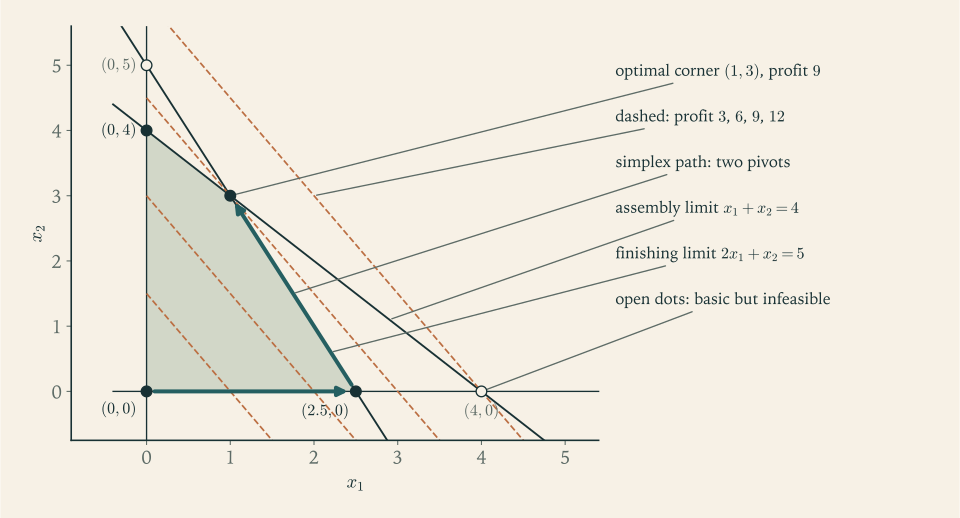
The workshop problem maximizes \(3x_1+2x_2\) subject to \(x_1+x_2\le 4\) , \(2x_1+x_2\le 5\) , and \(x\ge 0\) . Add a slack variable for each resource: \(x_3\) for unused assembly hours and \(x_4\) for unused finishing hours. Negating the objective, the standard form is
so that
Here \(m=2\) and \(n=4\) , and \(A\) has rank \(2\) . A point \((x_1,x_2)\) of the original quadrilateral corresponds to exactly one point \((x_1,x_2,\,4-x_1-x_2,\,5-2x_1-x_2)\) of the standard-form feasible set, and each side of the quadrilateral is the set where one of the four variables is zero. The plan \((1,3)\) becomes \(x=(1,3,0,0)\) and the plan \((0,0)\) becomes \(x=(0,0,4,5)\) .
4.2 Corners as basic feasible solutions
Definition 4.2 (extreme point). A point \(x\) of a convex set \(C\) is an extreme point, or vertex, of \(C\) if it is not the midpoint of two other points of \(C\) : whenever \(x=\tfrac12(u+v)\) with \(u,v\in C\) , necessarily \(u=v=x\) .
The definition is geometric. The next one is algebraic, and the theorem after it says they describe the same points.
Definition 4.3 (basis, basic feasible solution). For the standard-form constraints \(Ax=b\) , \(x\ge 0\) with \(A\) of rank \(m\) , a basis is a set \(B\) of \(m\) column indices such that the \(m\times m\) matrix \(A_B\) formed by those columns is invertible. The indices in \(B\) are basic and the remaining indices, collected in \(N\) , are nonbasic. The basic solution associated with \(B\) is the unique solution of \(Ax=b\) with \(x_N=0\) , namely
It is a basic feasible solution if in addition \(x_B\ge 0\) . A basic feasible solution is degenerate if some basic variable equals zero.
A basic solution is obtained by choosing which \(n-m\) variables to set to zero and solving for the rest. Geometrically, setting a variable to zero places the point on one face of the feasible region, and \(n-m\) such conditions together with the \(m\) equations pin down a single point.
Theorem 4.4 (vertices are basic feasible solutions). Let \(\mathcal F=\{x:Ax=b,\ x\ge 0\}\) with \(A\) of rank \(m\) , and let \(x\in\mathcal F\) . The following are equivalent: (a) \(x\) is an extreme point of \(\mathcal F\) ; (b) the columns of \(A\) corresponding to the positive components of \(x\) are linearly independent; (c) \(x\) is a basic feasible solution.
Proof. Let \(S=\{j:x_j>0\}\) be the support of \(x\) .
(b) implies (a). Suppose the columns indexed by \(S\) are independent and \(x=\tfrac12(u+v)\) with \(u,v\in\mathcal F\) . For \(j\notin S\) we have \(0=x_j=\tfrac12(u_j+v_j)\) with \(u_j,v_j\ge 0\) , so \(u_j=v_j=0\) . Then \(A(u-v)=b-b=0\) involves only the columns in \(S\) , and their independence forces \(u_j=v_j\) for \(j\in S\) as well. Hence \(u=v\) .
(a) implies (b). Suppose the columns indexed by \(S\) are dependent. Then there is \(w\ne 0\) with \(Aw=0\) and \(w_j=0\) for \(j\notin S\) . Since \(x_j>0\) on \(S\) , for small enough \(\varepsilon>0\) both \(x+\varepsilon w\) and \(x-\varepsilon w\) are nonnegative; both satisfy the equations because \(Aw=0\) . They are distinct points of \(\mathcal F\) with midpoint \(x\) , so \(x\) is not extreme.
(b) implies (c). The independent columns indexed by \(S\) number at most \(m\) . Because \(A\) has rank \(m\) , they can be extended by further columns of \(A\) to a set \(B\) of \(m\) independent columns. Then \(x_N=0\) , since \(N\) avoids \(S\) , and \(x\) solves \(Ax=b\) , so \(x\) is the basic solution for \(B\) , and it is feasible.
(c) implies (b). If \(x\) is the basic feasible solution for \(B\) , then \(S\subseteq B\) , and any subset of the independent columns \(A_B\) is independent.
Two consequences are immediate. There are at most \(\binom nm\) bases, so a polyhedron in standard form has finitely many vertices. And at a degenerate vertex, where \(S\) has fewer than \(m\) elements, the completion to a basis may fail to be unique, so that several bases represent one point (Exercise 8); whether it does depends on which other columns are independent of those in \(S\) .
Example 4.2: Every basis of the workshop problem
With \(m=2\) and \(n=4\) there are \(\binom42=6\) ways to choose two columns of the matrix \(A\) of Example 4.1, and every pair of its columns is independent. For each choice, set the other two variables to zero and solve.
| Basis | Basic solution \((x_1,x_2,x_3,x_4)\) | Feasible? | Point in the \((x_1,x_2)\) plane |
|---|---|---|---|
| \(\{1,2\}\) | \((1,3,0,0)\) | yes | \((1,3)\) |
| \(\{1,3\}\) | \((2.5,0,1.5,0)\) | yes | \((2.5,0)\) |
| \(\{1,4\}\) | \((4,0,0,-3)\) | no | \((4,0)\) |
| \(\{2,3\}\) | \((0,5,-1,0)\) | no | \((0,5)\) |
| \(\{2,4\}\) | \((0,4,0,1)\) | yes | \((0,4)\) |
| \(\{3,4\}\) | \((0,0,4,5)\) | yes | \((0,0)\) |
For instance, the basis \(\{1,3\}\) sets \(x_2=x_4=0\) ; the second equation gives \(2x_1=5\) , so \(x_1=2.5\) , and the first gives \(x_3=4-2.5=1.5\) . The four feasible rows are exactly the four corners of the quadrilateral. The two infeasible rows are the points where a resource line meets an axis outside the region: at \((4,0)\) the finishing constraint is violated by \(3\) hours, which is what \(x_4=-3\) records, and at \((0,5)\) assembly is over by \(1\) hour. No vertex is degenerate, because in each feasible row both basic variables are positive.
4.3 An optimal corner always exists
Theorem 4.5 (fundamental theorem of linear programming). Consider a linear program in standard form with \(A\) of rank \(m\) . (a) If the feasible set is nonempty, it has a basic feasible solution. (b) If the program has an optimal solution, it has an optimal solution that is a basic feasible solution.
Proof. We prove (b); part (a) is the same argument with \(c=0\) , for which every feasible point is optimal. Among all optimal solutions choose one, \(x\) , with the fewest positive components, and let \(S\) be its support. We claim the columns indexed by \(S\) are independent; Theorem 4.4 then shows that \(x\) is a basic feasible solution.
Suppose not. As in the proof of Theorem 4.4 there is \(w\ne 0\) with \(Aw=0\) and \(w_j=0\) off \(S\) , and \(x\pm\varepsilon w\) are feasible for small \(\varepsilon>0\) . Optimality of \(x\) gives \(c^{\top}(x\pm\varepsilon w)\ge c^{\top}x\) , so \(c^{\top}w\ge 0\) and \(c^{\top}w\le 0\) , that is, \(c^{\top}w=0\) . Replacing \(w\) by \(-w\) if necessary, some component of \(w\) is negative. Move from \(x\) in the direction \(w\) : the points \(x+tw\) satisfy \(Ax=b\) and have the same cost as \(x\) for every \(t\) . Increase \(t\) from \(0\) until the first component reaches zero, at \(t^\star=\min\{x_j/(-w_j):w_j<0\}>0\) . The point \(x+t^\star w\) is feasible, optimal, and has at least one fewer positive component than \(x\) , since its support lies in \(S\) and one index has dropped out. This contradicts the choice of \(x\) .
The theorem requires that an optimal solution exist. A linear program can also be infeasible, or unbounded below; what it cannot do is have a finite infimum that is not attained, a fact that will follow from the duality theorem. It also does not say that every optimal solution is a vertex. If the objective is parallel to an edge, every point of that edge is optimal, as in Exercise 1.13; the theorem promises that the edge’s endpoints are among the optima.
So the search for an optimum can be confined to a finite set. Finite does not mean small: with \(n=80\) and \(m=30\) there are about \(9\times 10^{21}\) candidate bases. An intelligent order of search is needed.
4.4 The simplex method
Fix a basis \(B\) with basic feasible solution \(x\) . The method needs two things: a test that recognises optimality, and, when the test fails, a neighbouring basis with a better cost.
Both come from one identity. For any vector \(y\in\mathbb R^m\) and any \(x'\) with \(Ax'=b\) ,
Choose \(y\) so that the coefficient vector \(c-A^{\top}y\) vanishes on the basic indices: solve \(A_B^{\top}y=c_B\) .
Definition 4.6 (reduced costs). For a basis \(B\) , let \(y\) be the solution of \(A_B^{\top}y=c_B\) . The vector \(\bar c=c-A^{\top}y\) is the vector of reduced costs. By construction \(\bar c_j=0\) for \(j\in B\) , and for nonbasic \(j\) , \(\bar c_j=c_j-y^{\top}A_j\) , where \(A_j\) is the \(j\) -th column of \(A\) .
With this \(y\) the identity reads
At the basic solution itself all nonbasic variables vanish, so its cost is \(c^{\top}x=y^{\top}b\) . The reduced cost \(\bar c_j\) is therefore the rate at which the total cost changes per unit increase of the nonbasic variable \(x_j\) , after the basic variables have been adjusted to keep \(Ax=b\) .
Theorem 4.7 (optimality test). Let \(x\) be a basic feasible solution with basis \(B\) and reduced costs \(\bar c\) . If \(\bar c\ge 0\) , then \(x\) is optimal.
Proof. For any feasible \(x'\) we have \(x'_j\ge 0\) , so the identity gives \(c^{\top}x'=y^{\top}b+\sum_{j\in N}\bar c_jx'_j\ge y^{\top}b=c^{\top}x\) .
If instead some reduced cost is negative, say \(\bar c_j<0\) with \(j\in N\) , increase \(x_j\) from zero to a value \(\theta\ge 0\) while holding the other nonbasic variables at zero. The equations force the basic variables to respond: from \(A_Bx_B+\theta A_j=b\) ,
and the cost becomes \(c^{\top}x+\theta\bar c_j\) , which decreases as \(\theta\) grows. How far can \(\theta\) grow? Basic variables with \(u_i\le 0\) do not decrease and impose no limit. A basic variable with \(u_i>0\) reaches zero when \(\theta\) equals its current value divided by \(u_i\) . Hence the ratio test
If no \(u_i\) is positive, \(\theta\) can grow without bound, the points \(x(\theta)\) remain feasible, and the cost tends to \(-\infty\) : the program is unbounded and the method has produced a ray that proves it. Otherwise, the basic variable attaining the minimum drops to zero and leaves the basis, the index \(j\) enters, and the new point is again a basic feasible solution, with cost lower by \(\theta^\star\lvert\bar c_j\rvert\) . That exchange is a pivot. The new columns are independent: replacing the leaving column by \(A_j=A_Bu\) keeps independence exactly because the coefficient \(u_i\) of the leaving column is nonzero.
The simplex method repeats this step. Start from a basic feasible solution. Compute \(y\) and the reduced costs. If none is negative, stop: the current vertex is optimal. Otherwise pick a nonbasic index with negative reduced cost, compute \(u\) , apply the ratio test, and pivot or report unboundedness.
Geometrically each pivot moves along an edge of the polyhedron from one vertex to an adjacent one with lower cost. If every vertex is nondegenerate then every \(\theta^\star\) is positive, the cost strictly decreases at each pivot, no basis can repeat, and since there are finitely many bases the method terminates. At a degenerate vertex \(\theta^\star\) can be zero: the basis changes but the point does not, and a careless choice of entering and leaving indices can cycle through the same bases forever. Cycling is prevented by a tie-breaking rule. Under Bland’s rule, which always chooses the eligible entering index and the eligible leaving index with the smallest subscript, the simplex method terminates after finitely many pivots on every linear program; we state this fact without proof. A starting basic feasible solution, when none is obvious, is found by applying the same method to an auxiliary program that minimizes the total violation of the constraints; this is called Phase I.
Example 4.3: Two pivots to the optimum
Apply the method to the standard form of Example 4.1, starting from the slack basis \(B=\{3,4\}\) , the vertex \((0,0)\) .
First pass. The basic solution is \(x_B=(x_3,x_4)=(4,5)\) with cost \(0\) . Since \(c_B=(0,0)\) , solving \(A_B^{\top}y=c_B\) gives \(y=(0,0)\) and the reduced costs are \(\bar c=c=(-3,-2,0,0)\) . Both nonbasic reduced costs are negative: making either product lowers the cost. Choose \(j=1\) . Then \(u=A_B^{-1}A_1=(1,2)\) , and the ratio test compares \(4/1\) with \(5/2\) . The minimum is \(\theta^\star=2.5\) , attained by \(x_4\) , which leaves. The new point is \(x=(2.5,0,1.5,0)\) with cost \(0+2.5\cdot(-3)=-7.5\) .
Second pass. Now \(B=\{1,3\}\) , \(A_B=\begin{pmatrix}1&1\\2&0\end{pmatrix}\) , \(c_B=(-3,0)\) . The system \(A_B^{\top}y=c_B\) reads \(y_1+2y_2=-3\) and \(y_1=0\) , so \(y=(0,-1.5)\) . The nonbasic reduced costs are \(\bar c_2=-2-(0\cdot 1-1.5\cdot 1)=-0.5\) and \(\bar c_4=0-(-1.5)=1.5\) . Index \(2\) enters. Solving \(A_Bu=A_2=(1,1)\) gives \(u=(0.5,0.5)\) for the basic variables \((x_1,x_3)=(2.5,1.5)\) ; the ratios are \(2.5/0.5=5\) and \(1.5/0.5=3\) , so \(\theta^\star=3\) and \(x_3\) leaves. The new point is \(x=(1,3,0,0)\) with cost \(-7.5+3\cdot(-0.5)=-9\) .
Third pass. Now \(B=\{1,2\}\) and \(c_B=(-3,-2)\) . The system \(y_1+2y_2=-3\) , \(y_1+y_2=-2\) gives \(y=(-1,-1)\) . The nonbasic reduced costs are \(\bar c_3=0-y_1=1\) and \(\bar c_4=0-y_2=1\) . Both are nonnegative, so by Theorem 4.7 the vertex \((1,3,0,0)\) is optimal, with cost \(-9\) , that is, profit \(9\) .
The method visited three of the four vertices, in the order \((0,0)\) , \((2.5,0)\) , \((1,3)\) , improving the profit from \(0\) to \(7.5\) to \(9\) . Had index \(2\) been chosen in the first pass, the path would have gone through \((0,4)\) instead.
4.5 Duality for linear programs
When the simplex method stops with \(\bar c\ge 0\) , the vector \(y\) it carries satisfies \(A^{\top}y\le c\) and \(y^{\top}b=c^{\top}x\) . Those two properties make \(y\) a proof of optimality that can be checked without rerunning the method. They are best understood through a second linear program.
Definition 4.8 (dual linear program). The dual of the standard-form program of Definition 4.1 is
with variable \(y\in\mathbb R^m\) unrestricted in sign. The original program is called the primal.
The dual has one variable for each primal equation and one inequality for each primal variable. Its origin is the search for lower bounds: if \(A^{\top}y\le c\) , then multiplying the \(j\) -th inequality by \(x_j\ge 0\) and adding shows that \(y^{\top}Ax\le c^{\top}x\) for every feasible \(x\) , and \(y^{\top}Ax=y^{\top}b\) . The dual asks for the best such bound.
Theorem 4.9 (weak duality for linear programs). If \(x\) is feasible for the primal and \(y\) is feasible for the dual, then \(b^{\top}y\le c^{\top}x\) . Consequently, if \(b^{\top}y=c^{\top}x\) for some feasible pair, then \(x\) is optimal for the primal and \(y\) is optimal for the dual.
Proof. \(c^{\top}x-b^{\top}y=c^{\top}x-y^{\top}Ax=(c-A^{\top}y)^{\top}x\ge 0\) , because both \(c-A^{\top}y\) and \(x\) are nonnegative vectors. If equality holds for the pair \((x,y)\) , then any primal feasible \(x'\) has \(c^{\top}x'\ge b^{\top}y=c^{\top}x\) and any dual feasible \(y'\) has \(b^{\top}y'\le c^{\top}x=b^{\top}y\) .
Theorem 4.10 (strong duality for linear programs). If the primal standard-form program has an optimal solution, then so does its dual, and the two optimal values are equal.
Proof. The primal is feasible, so by Theorem 4.5 it has a basic feasible solution from which the simplex method with Bland’s rule can start. The method terminates, and it cannot terminate with an unbounded ray because the primal has an optimal solution. So it terminates at a basis \(B\) with basic feasible solution \(x\) and reduced costs \(\bar c=c-A^{\top}y\ge 0\) , where \(A_B^{\top}y=c_B\) . The inequality \(\bar c\ge 0\) says \(A^{\top}y\le c\) : the vector \(y\) is dual feasible. And \(b^{\top}y=y^{\top}A_Bx_B=c_B^{\top}x_B=c^{\top}x\) . By Theorem 4.9 both are optimal, with equal values.
The proof is constructive: the simplex method solves both programs at once. It relies on the termination of the method under Bland’s rule, which we quoted. A consequence promised earlier follows: a feasible standard-form program whose objective is bounded below on the feasible set has an optimal solution, since the method must stop and cannot stop with a ray.
The term \((c-A^{\top}y)^{\top}x\) in the proof of weak duality is a sum of nonnegative products, and that observation gives a third characterization of optimality.
Theorem 4.11 (complementary slackness). Let \(x\) be primal feasible and \(y\) dual feasible. Then both are optimal if and only if
Proof. The duality gap is \(c^{\top}x-b^{\top}y=\sum_jx_j(c_j-A_j^{\top}y)\) , a sum of nonnegative terms. It is zero if and only if every term is zero. If the gap is zero both are optimal by Theorem 4.9; if both are optimal the gap is zero by Theorem 4.10.
In words: for each \(j\) , either the primal variable \(x_j\) is zero or the \(j\) -th dual constraint holds with equality. A positive primal variable forces its dual constraint to be tight; a slack dual constraint forces its primal variable to vanish.
A triple of checks, primal feasibility, dual feasibility, and equal objective values, is called a primal–dual certificate of optimality. Its value is that it separates finding a solution from verifying one. Verification needs no knowledge of how the pair was produced, only a handful of matrix products and comparisons.
For a program given in inequality form the dual takes a symmetric shape. The pair
is obtained by putting the first program into standard form with slack variables, writing the dual by Definition 4.8, and replacing its variable by its negative; Exercise 5 asks for the direct proof of weak duality for this pair. In this form the dual variables are nonnegative shadow prices, one per resource.
The possible outcomes for a primal and dual pair are limited by weak duality. If the primal is unbounded, the dual has no feasible point, since any dual feasible \(y\) would bound the primal from below. If both are feasible, both have optimal solutions with equal values. It is also possible for both to be infeasible.
Example 4.4: The workshop’s dual and its shadow prices
In inequality form the workshop problem maximizes \(3x_1+2x_2\) subject to \(x_1+x_2\le 4\) , \(2x_1+x_2\le 5\) , \(x\ge 0\) . Its dual attaches a price \(y_1\) to an assembly hour and \(y_2\) to a finishing hour:
The dual constraints say that the resources consumed by one unit of each product must be valued at no less than that product’s profit; the dual objective is the total value of the available resources at those prices.
At the primal optimum \(x=(1,3)\) both variables are positive, so complementary slackness forces both dual constraints to be tight: \(y_1+2y_2=3\) and \(y_1+y_2=2\) , giving \(y=(1,1)\) . This is feasible, and its objective value is \(4+5=9\) , equal to the primal profit. The certificate is complete: \(x=(1,3)\) is primal feasible with value \(9\) , \(y=(1,1)\) is dual feasible with value \(9\) , so both are optimal. The simplex multipliers \(y=(-1,-1)\) of Example 4.3 are the same prices with the sign that the minimization form imposes.
The prices predict how the optimal profit responds to the resource limits. With \(5\) assembly hours in place of \(4\) , re-solving gives the plan \((0,5)\) with profit \(10\) , an increase of \(1=y_1\) . With \(6\) finishing hours in place of \(5\) , re-solving gives the plan \((2,2)\) with profit \(10\) , an increase of \(1=y_2\) . An extra hour of either resource is worth exactly its shadow price, as long as the change does not alter which constraints are active.
Example 4.5: An unbounded program and its infeasible dual
Maximize \(x_1+x_2\) subject to \(x_1-x_2\le 1\) and \(x\ge 0\) . In standard form: minimize \(-x_1-x_2\) subject to \(x_1-x_2+x_3=1\) , \(x\ge 0\) , with the single slack \(x_3\) . Start from the basis \(\{3\}\) , where \(x=(0,0,1)\) , \(y=0\) , and \(\bar c=(-1,-1,0)\) . Let index \(2\) enter. Then \(u=A_B^{-1}A_2=-1\) , which is not positive: increasing \(x_2\) makes the basic variable \(x_3=1+x_2\) grow, so the ratio test finds no limit. The points \((0,\theta,1+\theta)\) are feasible for every \(\theta\ge 0\) with cost \(-\theta\) . The program is unbounded, and the ray \((0,\theta)\) in the original variables proves it.
The dual in inequality form is: minimize \(y\) subject to \(y\ge 1\) (from the column of \(x_1\) ), \(-y\ge 1\) (from the column of \(x_2\) ), \(y\ge 0\) . The second constraint demands \(y\le-1\) , which contradicts \(y\ge 0\) . The dual is infeasible, as weak duality requires.
Common mistake. Accepting a dual vector as a certificate because the objective values agree, without checking dual feasibility. At the workshop vertex \((2.5,0)\) the simplex multipliers correspond to prices \(y=(0,1.5)\) , and the values agree: \(4\cdot 0+5\cdot 1.5=7.5=3\cdot 2.5\) . Complementary slackness holds too. But \(y_1+y_2=1.5<2\) , so the second dual constraint fails and \(y\) is not dual feasible. Agreement of values at every basis is automatic, by the identity \(c^{\top}x=y^{\top}b\) ; it is feasibility of both vectors that carries the information. A negative reduced cost and a violated dual constraint are the same thing.
4.6 Quadratic programs
Definition 4.12 (quadratic program). A quadratic program minimizes a quadratic function \(\tfrac12x^{\top}Px+q^{\top}x\) , with \(P\) symmetric, subject to finitely many affine equality and inequality constraints. It is a convex quadratic program if \(P\succeq 0\) .
By Theorem 2.6 the objective is convex exactly when \(P\succeq 0\) , and the feasible set is a polyhedron, so a convex quadratic program is a convex optimization problem. Unlike a linear program, its solution need not be at a vertex: the minimizer of \((x_1-2)^2+(x_2-2)^2\) over the workshop quadrilateral lies in the middle of an edge (Exercise 20). With inequality constraints the difficulty is to discover which of them are active, and that is the subject of Chapter 6. With equality constraints only, the problem reduces to linear algebra.
Consider minimizing \(f(x)=\tfrac12x^{\top}Px+q^{\top}x\)
subject to \(Ax=b\)
, where \(A\)
is \(p\times n\)
. The method of Lagrange multipliers from multivariable calculus (math.multivariable-calculus.lagrange-multiplier) says that at a constrained minimizer the gradient of the objective is a combination of the gradients of the constraints. Here the gradient of \(f\)
is \(Px+q\)
and the constraint gradients are the rows of \(A\)
, so the condition is \(Px+q+A^{\top}\nu=0\)
for some \(\nu\in\mathbb R^p\)
. Together with feasibility this is a square linear system in \((x,\nu)\)
:
For a quadratic objective we need not take the multiplier rule on trust. The following theorem proves directly that a solution of the system is a minimizer, and says when.
Theorem 4.13 (equality-constrained quadratic program). Let \(P\) be symmetric and suppose \((x^\star,\nu^\star)\) satisfies \(Px^\star+q+A^{\top}\nu^\star=0\) and \(Ax^\star=b\) .
(a) If \(d^{\top}Pd\ge 0\) for every \(d\) in the null space of \(A\) , then \(x^\star\) minimizes \(f\) over \(\{x:Ax=b\}\) .
(b) If \(d^{\top}Pd>0\) for every nonzero \(d\) in the null space of \(A\) , then \(x^\star\) is the unique minimizer.
(c) If the hypothesis of (b) holds and \(A\) has full row rank, the coefficient matrix of the system is invertible, so \((x^\star,\nu^\star)\) exists and is unique.
Proof. Any feasible point is \(x^\star+d\) with \(Ad=0\) . Expanding the quadratic and using \(Px^\star+q=-A^{\top}\nu^\star\) ,
Parts (a) and (b) follow at once. For (c) it suffices to show that the homogeneous system has only the zero solution. If \(Pv+A^{\top}w=0\) and \(Av=0\) , then \(v^{\top}Pv=-v^{\top}A^{\top}w=-(Av)^{\top}w=0\) ; since \(v\) lies in the null space of \(A\) , hypothesis (b) forces \(v=0\) . Then \(A^{\top}w=0\) , and full row rank of \(A\) forces \(w=0\) .
The hypotheses concern \(P\)
only on the null space of \(A\)
, the set of directions in which one can move while staying feasible (math.linear-algebra.null-space-meaning). A matrix can be indefinite on \(\mathbb R^n\)
and positive definite on that subspace, in which case the unconstrained problem is unbounded and the constrained one is perfectly well posed.
Example 4.6: Two equality-constrained problems
Nearest point on a line. Minimize \(x^2+y^2\) subject to \(x+y=1\) . Here \(P=2I\) , \(q=0\) , \(A=\begin{pmatrix}1&1\end{pmatrix}\) , \(b=1\) . The system is \(2x+\nu=0\) , \(2y+\nu=0\) , \(x+y=1\) . The first two equations give \(x=y\) , and the third gives \(x=y=\tfrac12\) with \(\nu=-1\) . Since \(P\) is positive definite, Theorem 4.13 says \((\tfrac12,\tfrac12)\) is the unique minimizer; the optimal value is \(\tfrac12\) . Substituting \(y=1-x\) and minimizing \(x^2+(1-x)^2\) gives the same point.
A minimum-variance portfolio. Two assets have covariance matrix \(\Sigma=\begin{pmatrix}4&1\\1&2\end{pmatrix}\) . Minimize the variance \(x^{\top}\Sigma x\) of a portfolio with weights \(x\) subject to \(x_1+x_2=1\) . Scaling the objective by \(\tfrac12\) does not change the minimizer, so take \(P=\Sigma\) , \(q=0\) . The system is
Subtracting the second equation from the first gives \(3x_1-x_2=0\) , so \(x_2=3x_1\) and then \(x^\star=(\tfrac14,\tfrac34)\) , with \(\nu^\star=-\tfrac74\) . The variance is \(x^{\star\top}\Sigma x^\star=\tfrac14+\tfrac38+\tfrac98=\tfrac74\) , lower than the variance \(2\) of the less risky asset held alone. Three quarters of the portfolio goes to the low-variance asset, but not all of it: the imperfect correlation makes some diversification worthwhile.
Example 4.7: A negative eigenvalue blocked by a constraint
Let \(f(x)=\tfrac12(x_1^2-x_2^2)\) , so \(P\) is diagonal with entries \(1\) and \(-1\) . By Theorem 3.7(c) the unconstrained problem is unbounded below: along the eigenvector \((0,1)\) the function is \(-\tfrac12t^2\) .
Now impose \(x_1-2x_2=1\) . The null space of \(A=\begin{pmatrix}1&-2\end{pmatrix}\) is spanned by \(d=(2,1)\) , and \(d^{\top}Pd=4-1=3>0\) . The matrix \(P\) is positive definite on the feasible directions, and Theorem 4.13 applies. The system
gives \(x_1=-\nu\) , \(x_2=-2\nu\) , and then \(-\nu+4\nu=1\) , so \(\nu^\star=\tfrac13\) and \(x^\star=(-\tfrac13,-\tfrac23)\) , with \(f(x^\star)=\tfrac12(\tfrac19-\tfrac49)=-\tfrac16\) . Along the feasible line \(x=x^\star+t(2,1)\) the objective is \(-\tfrac16+\tfrac32t^2\) , an upward parabola. The direction of negative curvature \((0,1)\) is not a feasible direction, so the constraint has removed it from the problem.
Had the constraint been \(x_1=1\) , with feasible direction \((0,1)\) , the curvature along the feasible line would be \(-1\) and the constrained problem would remain unbounded. Convexity of a constrained problem is decided on the feasible directions, not on the whole space.
Linear programs came with a dual program whose solutions certify optimality, and equality-constrained quadratic programs came with multipliers \(\nu\) . These are two views of one construction. The next chapter builds it for a general problem: a Lagrangian that prices each constraint, and a dual function whose values bound the optimum from below whatever the problem’s shape.
Exercises
-
Put the program “maximize \(2x_1-x_2\) subject to \(x_1+x_2\ge 2\) , \(x_1-x_2\le 3\) , \(x_1\ge 0\) , with \(x_2\) unrestricted in sign” into standard form, listing the new variables and writing out \(A\) , \(b\) , and \(c\) .
Answer
Write \(x_2=x_2^+-x_2^-\) with \(x_2^+,x_2^-\ge 0\) , subtract a surplus variable \(s_1\ge 0\) in the first constraint, and add a slack \(s_2\ge 0\) in the second. In the variable order \((x_1,x_2^+,x_2^-,s_1,s_2)\) : minimize \(c^{\top}x\) with \(c=(-2,1,-1,0,0)\) subject to \(Ax=b\) , \(x\ge 0\) , where \(A=\begin{pmatrix}1&1&-1&-1&0\\1&-1&1&0&1\end{pmatrix}\) and \(b=(2,3)\) .
-
For the constraints \(x_1+x_2+x_3=4\) , \(x_1+2x_2+x_4=6\) , \(x\ge 0\) , list all six bases with their basic solutions, mark which are feasible, and identify the corresponding points of the \((x_1,x_2)\) plane.
Solution
Here \(A=\begin{pmatrix}1&1&1&0\\1&2&0&1\end{pmatrix}\) and \(b=(4,6)\) . Each pair of columns is independent, so there are six bases. For each, set the two nonbasic variables to zero and solve the two equations.
Basis \(\{1,2\}\) : \(x_1+x_2=4\) and \(x_1+2x_2=6\) give \(x_2=2\) , \(x_1=2\) ; solution \((2,2,0,0)\) , feasible, the point \((2,2)\) . Basis \(\{1,3\}\) : \(x_1=6\) from the second equation, then \(x_3=4-6=-2\) ; solution \((6,0,-2,0)\) , infeasible, the point \((6,0)\) . Basis \(\{1,4\}\) : \(x_1=4\) , then \(x_4=6-4=2\) ; solution \((4,0,0,2)\) , feasible, the point \((4,0)\) . Basis \(\{2,3\}\) : \(x_2=3\) , then \(x_3=4-3=1\) ; solution \((0,3,1,0)\) , feasible, the point \((0,3)\) . Basis \(\{2,4\}\) : \(x_2=4\) , then \(x_4=6-8=-2\) ; solution \((0,4,0,-2)\) , infeasible, the point \((0,4)\) . Basis \(\{3,4\}\) : solution \((0,0,4,6)\) , feasible, the point \((0,0)\) .
The four basic feasible solutions are the vertices \((0,0)\) , \((4,0)\) , \((2,2)\) , \((0,3)\) of the region \(x_1+x_2\le 4\) , \(x_1+2x_2\le 6\) , \(x\ge 0\) , in agreement with Theorem 4.4. The two infeasible basic solutions are the intersections of each constraint line with the axis on which the other constraint is violated.
-
Solve “maximize \(2x_1+3x_2\) subject to \(x_1+x_2\le 4\) , \(x_1+2x_2\le 6\) , \(x\ge 0\) ” by the simplex method starting from the slack basis, reporting \(y\) , the reduced costs, the entering and leaving variables, and the cost at every pass.
Solution
Standard form: minimize \(-2x_1-3x_2\) subject to \(x_1+x_2+x_3=4\) , \(x_1+2x_2+x_4=6\) , \(x\ge 0\) , so \(c=(-2,-3,0,0)\) .
Pass 1. Basis \(\{3,4\}\) , \(x_B=(4,6)\) , cost \(0\) , \(y=(0,0)\) , \(\bar c=(-2,-3,0,0)\) . Let index \(2\) enter (the most negative reduced cost). \(u=A_B^{-1}A_2=(1,2)\) ; ratios \(4/1=4\) and \(6/2=3\) ; \(\theta^\star=3\) and \(x_4\) leaves. New point \((0,3,1,0)\) , cost \(0+3\cdot(-3)=-9\) .
Pass 2. Basis \(\{3,2\}\) with \(c_B=(0,-3)\) . Solve \(A_B^{\top}y=c_B\) : the column of \(x_3\) gives \(y_1=0\) and the column of \(x_2\) gives \(y_1+2y_2=-3\) , so \(y=(0,-1.5)\) . Reduced costs: \(\bar c_1=-2-(y_1+y_2)=-0.5\) and \(\bar c_4=0-y_2=1.5\) . Index \(1\) enters. Solving \(A_Bu=A_1\) for the basic variables \((x_3,x_2)\) : from the second equation \(2u_2=1\) , so \(u_2=0.5\) , and from the first \(u_1+u_2=1\) , so \(u_1=0.5\) . Ratios: \(1/0.5=2\) for \(x_3\) and \(3/0.5=6\) for \(x_2\) ; \(\theta^\star=2\) and \(x_3\) leaves. New point \((2,2,0,0)\) , cost \(-9+2\cdot(-0.5)=-10\) .
Pass 3. Basis \(\{1,2\}\) with \(c_B=(-2,-3)\) : \(y_1+y_2=-2\) and \(y_1+2y_2=-3\) give \(y=(-1,-1)\) . Reduced costs: \(\bar c_3=0-y_1=1\) and \(\bar c_4=0-y_2=1\) . Both are nonnegative, so by Theorem 4.7 the vertex is optimal. The maximum of \(2x_1+3x_2\) is \(10\) , attained at \((x_1,x_2)=(2,2)\) . The path was \((0,0)\to(0,3)\to(2,2)\) .
-
Write the dual of the program in Exercise 3 in inequality form, find its optimal solution using complementary slackness with the primal optimum, and assemble the primal–dual certificate.
Solution
By the inequality-form rule of Section 4.5 the dual is
\[ \begin{aligned} \text{minimize}\quad & 4y_1+6y_2\\ \text{subject to}\quad & y_1+y_2\ge 2,\quad y_1+2y_2\ge 3,\quad y\ge 0 . \end{aligned} \]The primal optimum is \(x=(2,2)\) with both components positive, so by complementary slackness both dual constraints must hold with equality: \(y_1+y_2=2\) and \(y_1+2y_2=3\) . Subtracting gives \(y_2=1\) , hence \(y_1=1\) . Both primal constraints are active at \((2,2)\) , so complementary slackness places no further restriction on \(y\) .
Certificate. Primal feasibility: \(2+2=4\le 4\) , \(2+4=6\le 6\) , \(x\ge 0\) . Dual feasibility: \(1+1=2\ge 2\) , \(1+2=3\ge 3\) , \(y\ge 0\) . Equal values: \(2\cdot2+3\cdot2=10\) and \(4\cdot1+6\cdot1=10\) . By weak duality both are optimal. The dual solution is the negative of the final simplex multiplier \(y=(-1,-1)\) of Exercise 4.3, as expected from the sign change between the minimization and maximization forms.
-
Prove weak duality directly for the inequality-form pair: if \(Ax\le b\) , \(x\ge 0\) , \(A^{\top}y\ge c\) , \(y\ge 0\) , then \(c^{\top}x\le b^{\top}y\) ; state at which step each of the four hypotheses is used.
Hint
Chain two inequalities: \(c^{\top}x\le(A^{\top}y)^{\top}x\) uses \(A^{\top}y\ge c\) together with \(x\ge 0\) ; then \((A^{\top}y)^{\top}x=y^{\top}(Ax)\le y^{\top}b\) uses \(Ax\le b\) together with \(y\ge 0\) .
-
For the workshop problem a colleague offers the plan \(x=(2.5,0)\) with prices \(y=(0,1.5)\) as a primal–dual certificate, pointing out that \(3\cdot2.5=7.5=4\cdot0+5\cdot1.5\) and that complementary slackness holds. Check each requirement of a certificate, identify the one that fails, and explain what the failure says about the reduced costs at that vertex.
Solution
A primal–dual certificate has three parts. Primal feasibility of \(x=(2.5,0)\) : \(2.5\le 4\) , \(5\le 5\) , \(x\ge 0\) ; this holds. Equal objective values: \(7.5=7.5\) ; this holds. Dual feasibility of \(y=(0,1.5)\) for the dual of Example 4.4: the first constraint is \(y_1+2y_2=3\ge 3\) , which holds, but the second is \(y_1+y_2=1.5\ge 2\) , which fails. So the offered pair is not a certificate, and weak duality gives no conclusion; indeed \((2.5,0)\) is not optimal, since \((1,3)\) has profit \(9\) .
Agreement of the objective values proves nothing by itself. At any basis the simplex multipliers satisfy \(y^{\top}b=c^{\top}x\) identically, and complementary slackness between \(x\) and the reduced costs holds at every basis too, because reduced costs vanish on basic indices and nonbasic variables are zero. The only condition that distinguishes an optimal basis is the sign of the reduced costs. The violated dual constraint is the one belonging to the column of \(x_2\) , and its violation \(2-1.5=0.5\) is exactly the negative reduced cost \(\bar c_2=-0.5\) found in the second pass of Example 4.3. A violated dual constraint identifies a variable worth bringing into the basis.
-
Show that “maximize \(x_1+x_2\) subject to \(x_1-x_2\le 1\) , \(-x_1+x_2\le 1\) , \(x\ge 0\) ” is unbounded by exhibiting a feasible ray, and show by adding its two constraints that its dual is infeasible.
Answer
The points \((t,t)\) with \(t\ge 0\) are feasible, since \(t-t=0\le 1\) in both constraints, and the objective \(2t\) is unbounded. The dual is: minimize \(y_1+y_2\) subject to \(y_1-y_2\ge 1\) , \(-y_1+y_2\ge 1\) , \(y\ge 0\) . Adding the two constraints gives \(0\ge 2\) , so no \(y\) is feasible.
-
The constraints \(x_1+x_2\le 2\) , \(x_1\le 2\) , \(x\ge 0\) have a vertex at \((2,0)\) where three of the four inequalities are active. Put the constraints in standard form, find every basis whose basic solution is that vertex, and say why the vertex is called degenerate.
Answer
Standard form: \(x_1+x_2+x_3=2\) , \(x_1+x_4=2\) , \(x\ge 0\) . The vertex is \(x=(2,0,0,0)\) . Its support is \(\{1\}\) , a single independent column, which can be completed to a basis by adding column \(2\) , \(3\) , or \(4\) ; each of \(\{1,2\}\) , \(\{1,3\}\) , \(\{1,4\}\) is a basis with that same basic solution. It is degenerate because a basic variable equals zero in each case; equivalently, more than \(n-m=2\) of the sign constraints are active.
-
Prove that a nonempty feasible set \(\{x:Ax=b,\ x\ge 0\}\) has at least one extreme point, show that the halfplane \(\{x\in\mathbb R^2:x_1+x_2\le 1\}\) has none, and explain which feature of standard form accounts for the difference.
Hint
Existence is Theorem 4.5(a) combined with Theorem 4.4. For the halfplane, any point is the midpoint of two others obtained by moving in the directions \(\pm(1,-1)\) , which stay in the set. A set that contains a whole line has no extreme points, and \(x\ge 0\) prevents a standard-form feasible set from containing a line.
-
Let \(x\) be a basic feasible solution whose nonbasic reduced costs are all strictly positive. Prove that \(x\) is the unique optimal solution, and show by example that uniqueness can fail when a nonbasic reduced cost is zero.
Solution
Let \(B\) be the basis, \(y\) the solution of \(A_B^{\top}y=c_B\) , and \(\bar c=c-A^{\top}y\) . For every feasible \(x'\) , the identity of Section 4.4 gives
\[ c^{\top}x'=c^{\top}x+\sum_{j\in N}\bar c_jx'_j . \]By Theorem 4.7 the point \(x\) is optimal, since \(\bar c\ge 0\) . Suppose \(x'\) is also optimal. Then \(c^{\top}x'=c^{\top}x\) , so \(\sum_{j\in N}\bar c_jx'_j=0\) . Every term is a product of a strictly positive number \(\bar c_j\) and a nonnegative number \(x'_j\) , so every \(x'_j\) with \(j\in N\) must be zero. Then \(A_Bx'_B=b\) , and since \(A_B\) is invertible, \(x'_B=A_B^{-1}b=x_B\) . Hence \(x'=x\) .
If some nonbasic reduced cost is zero, uniqueness can fail. For the objective “maximize \(2x_1+x_2\) ” over the workshop constraints, the basis \(\{1,2\}\) at the vertex \((1,3)\) has reduced costs \(\bar c_3=0\) and \(\bar c_4=1\) (Exercise 4.19). Increasing \(x_3\) from zero moves along the edge toward \((2.5,0)\) without changing the cost, and every point of that edge is optimal with value \(5\) . Note that the proof used no nondegeneracy assumption: strict positivity of the nonbasic reduced costs suffices for uniqueness of the optimal solution, although at a degenerate vertex the basis representing it need not be unique.
-
In Example 4.4 the shadow price of assembly is \(1\) . Predict the optimal profit when the assembly limit is \(4.5\) hours, verify the prediction by solving the modified program, and find the largest assembly limit up to which the prediction rule “profit increases by \(1\) per extra hour” remains valid.
Solution
The shadow price \(y_1=1\) predicts that half an extra assembly hour raises the profit by \(0.5\) , to \(9.5\) .
To verify, solve with limits \((4.5,5)\) . If both resource constraints stay active, \(x_1+x_2=4.5\) and \(2x_1+x_2=5\) give \(x_1=0.5\) and \(x_2=4\) , which is nonnegative, hence a vertex; its profit is \(1.5+8=9.5\) . The prices \(y=(1,1)\) are still dual feasible, because the dual constraints do not involve the resource limits, and the dual value is \(4.5+5=9.5\) . Equal values certify optimality, and the prediction is confirmed.
For a general assembly limit \(\beta\) , the vertex with both resource constraints active is \(x_1=5-\beta\) , \(x_2=2\beta-5\) , with profit \(3(5-\beta)+2(2\beta-5)=5+\beta\) . It is feasible while \(x_1\ge 0\) and \(x_2\ge 0\) , that is, for \(2.5\le\beta\le 5\) . On that range the profit is \(5+\beta\) , increasing by exactly \(1\) per hour. At \(\beta=5\) the vertex reaches \((0,5)\) ; for larger \(\beta\) the assembly constraint is no longer active, the optimal plan stays at \((0,5)\) with profit \(10\) , and the shadow price of assembly drops to \(0\) . The largest limit for which the rule is valid is \(5\) hours.
-
Minimize \(x_1^2+2x_2^2+x_3^2\) subject to \(x_1+x_2+x_3=4\) by solving the linear system of Theorem 4.13, and state which part of that theorem guarantees that your solution is the unique minimizer.
Solution
Here \(P\) is diagonal with entries \(2,4,2\) , \(q=0\) , \(A=\begin{pmatrix}1&1&1\end{pmatrix}\) , and \(b=4\) . The system \(Px+A^{\top}\nu=0\) , \(Ax=b\) reads
\[ 2x_1+\nu=0,\qquad 4x_2+\nu=0,\qquad 2x_3+\nu=0,\qquad x_1+x_2+x_3=4 . \]So \(x_1=x_3=-\nu/2\) and \(x_2=-\nu/4\) . Substituting into the constraint, \(-\tfrac54\nu=4\) , so \(\nu^\star=-3.2\) and \(x^\star=(1.6,\ 0.8,\ 1.6)\) . The optimal value is \(2.56+1.28+2.56=6.4\) .
The matrix \(P\) is positive definite on all of \(\mathbb R^3\) , hence on the null space of \(A\) , so part (b) of Theorem 4.13 gives uniqueness; \(A\) has full row rank, so part (c) guarantees that the system has exactly one solution. The variable with the larger cost coefficient receives the smaller share, and the products \(2x_1\) , \(4x_2\) , \(2x_3\) are all equal to \(-\nu^\star=3.2\) : at the optimum the marginal cost of every variable is the same.
-
The system of Theorem 4.13 for “minimize \(x_1x_2\) subject to \(x_1+x_2=2\) ” has the solution \(x=(1,1)\) , \(\nu=-1\) . Decide whether \((1,1)\) is a minimizer by examining \(d^{\top}Pd\) on the null space of \(A\) , and describe the behaviour of the objective along the feasible line.
Solution
Write \(x_1x_2=\tfrac12x^{\top}Px\) with \(P=\begin{pmatrix}0&1\\1&0\end{pmatrix}\) , and \(A=\begin{pmatrix}1&1\end{pmatrix}\) . The system is \(x_2+\nu=0\) , \(x_1+\nu=0\) , \(x_1+x_2=2\) , with solution \(x=(1,1)\) , \(\nu=-1\) , as stated.
The null space of \(A\) is spanned by \(d=(1,-1)\) , and \(d^{\top}Pd=-2<0\) . Neither hypothesis (a) nor (b) of Theorem 4.13 holds, so the theorem does not make \((1,1)\) a minimizer. The expansion in its proof still applies and tells the whole story: along the feasible line \(x=(1+t,\,1-t)\) the objective is \(f=(1+t)(1-t)=1-t^2\) . It has a maximum at \(t=0\) and tends to \(-\infty\) as \(t\to\pm\infty\) . So \((1,1)\) is the constrained maximizer, and the minimization problem is unbounded below. Solving the multiplier system finds stationary points of the objective on the feasible set; whether such a point is a minimizer, a maximizer, or neither is decided by the curvature on the feasible directions, and that check cannot be skipped.
-
Solve the portfolio problem of Example 4.6 a second way, by writing every feasible point as \(x=(1,0)+w(-1,1)\) and minimizing over the scalar \(w\) , and confirm that the two methods agree.
Answer
With \(x=(1-w,\,w)\) the variance is \(4(1-w)^2+2(1-w)w+2w^2=4w^2-6w+4\) , minimized at \(w=\tfrac34\) with value \(\tfrac94-\tfrac92+4=\tfrac74\) . This is \(x=(\tfrac14,\tfrac34)\) , as in Example 4.6.
-
Two plants can supply 20 and 30 units and three markets demand 10, 25, and 15 units; shipping one unit from plant \(i\) to market \(j\) costs \(c_{ij}\) . Formulate the cheapest shipping plan as a linear program in standard form, count its variables and equations, and explain why its constraint matrix has rank 4 and not 5.
Hint
Use six variables \(x_{ij}\ge 0\) . Total supply equals total demand, \(50\) , so all five constraints can be written as equations: two supply equations and three demand equations. The sum of the supply equations equals the sum of the demand equations, so one equation is redundant; any four are independent. Delete one to meet the full-row-rank assumption.
-
Show that the optimal set of any linear program is convex, and use Theorem 2.10 to explain why a vertex whose cost is no larger than that of every point on the edges leaving it must be globally optimal.
Hint
The optimal set is the intersection of the feasible polyhedron with the hyperplane \(\{x:c^{\top}x=p^\star\}\) . For the second part, use the fact that near a vertex every feasible direction is a nonnegative combination of the directions of the edges leaving it; a linear cost that does not decrease along any edge then does not decrease along any feasible direction, so the vertex is a local minimizer.
-
Starting from the vertex \((0,4)\) of the workshop problem, with basis \(\{2,4\}\) , carry out one simplex pivot: compute \(y\) , the reduced costs, the vector \(u\) , the ratio test, and the new vertex and cost.
Answer
\(A_B\) has columns \(A_2=(1,1)\) and \(A_4=(0,1)\) , \(c_B=(-2,0)\) , so \(y_1+y_2=-2\) , \(y_2=0\) , giving \(y=(-2,0)\) . Reduced costs: \(\bar c_1=-3-(-2)=-1\) , \(\bar c_3=0-(-2)=2\) . Index \(1\) enters; \(u=(1,1)\) for the basic variables \((x_2,x_4)=(4,1)\) ; ratios \(4\) and \(1\) ; \(\theta^\star=1\) and \(x_4\) leaves. New vertex \((1,3,0,0)\) with cost \(-8+1\cdot(-1)=-9\) .
-
Show that the dual of the dual is the primal for the inequality-form pair of Section 4.5, by rewriting the dual as a maximization in inequality form and applying the same rule again.
Hint
Rewrite “minimize \(b^{\top}y\) subject to \(A^{\top}y\ge c\) , \(y\ge 0\) ” as “maximize \((-b)^{\top}y\) subject to \((-A^{\top})y\le-c\) , \(y\ge 0\) ”, apply the rule to get “minimize \((-c)^{\top}x\) subject to \((-A)x\ge-b\) , \(x\ge 0\) ”, and simplify the signs.
-
For the objective “maximize \(2x_1+x_2\) ” over the workshop constraints, compute the reduced costs at the basis \(\{1,2\}\) , observe that one nonbasic reduced cost is zero, and identify all optimal solutions.
Answer
With \(c=(-2,-1,0,0)\) and \(B=\{1,2\}\) : \(y_1+2y_2=-2\) , \(y_1+y_2=-1\) , so \(y=(0,-1)\) and \(\bar c_3=0\) , \(\bar c_4=1\) . The vertex \((1,3)\) is optimal with value \(5\) , and because \(\bar c_3=0\) the adjacent vertex \((2.5,0)\) has the same value. The optimal set is the whole edge between \((1,3)\) and \((2.5,0)\) .
-
Find the minimizer of \((x_1-2)^2+(x_2-2)^2\) over the workshop quadrilateral by projecting \((2,2)\) onto the line \(2x_1+x_2=5\) and checking the remaining constraints, and explain why the fact that the minimizer is not a vertex does not contradict Theorem 4.5.
Solution
The objective is the squared distance from the point \((2,2)\) , which violates the finishing constraint since \(2\cdot2+2=6>5\) . Consider first the relaxed problem of minimizing over the single halfplane \(H=\{x:2x_1+x_2\le 5\}\) . The nearest point of \(H\) to an outside point lies on the boundary line and is the foot of the perpendicular:
\[ x=(2,2)-\frac{2\cdot 2+2-5}{2^2+1^2}\,(2,1)=(2,2)-\tfrac15(2,1)=(1.6,\ 1.8). \]Check the constraints that were dropped: \(1.6+1.8=3.4\le 4\) , and both coordinates are nonnegative. So \((1.6,1.8)\) lies in the workshop quadrilateral, which is a subset of \(H\) . By Proposition 1.8, a minimizer of the relaxed problem that is feasible for the original problem is optimal for it. The minimizer is \((1.6,1.8)\) , with value \(0.4^2+0.2^2=0.2\) .
This point is in the relative interior of the edge joining \((2.5,0)\) and \((1,3)\) ; it is not a vertex. There is no contradiction with Theorem 4.5, which concerns linear objectives. The level sets of a linear objective are hyperplanes, and a hyperplane leaving a polyhedron last touches it at a face that contains a vertex. The level sets here are circles, and a circle can touch an edge at an interior point. For a quadratic program the number of active constraints at the solution is not known in advance, which is why the vertex-enumeration idea behind the simplex method does not carry over directly.