A small workshop makes two products. Each unit of the first earns a profit of 3 and each unit of the second a profit of 2. A unit of either product needs one hour of assembly, and 4 assembly hours are available per day; a unit of the first needs two hours on a finishing machine, a unit of the second needs one, and the machine runs 5 hours per day. How much of each product should the workshop make?
The question sounds like arithmetic, yet it hides three separate issues that recur in every optimization problem. First, what exactly is being chosen, and which choices are allowed? Second, is there a best choice at all, or only a sequence of ever better ones? Third, if the same question is written down in two different ways, do the two formulations have the same answers? This chapter supplies the vocabulary for all three, proves the basic existence theorem, and develops the geometric picture of objective level sets sliding across a feasible region that the remaining chapters turn into theorems and algorithms.
1.1 The parts of a problem
Definition 1.1 (optimization problem in standard form). Let \(f_0,f_1,\dots,f_m\) and \(h_1,\dots,h_p\) be real-valued functions defined on a common domain \(\mathcal D\subseteq\mathbb R^n\) . The associated optimization problem is
The vector \(x\in\mathbb R^n\) is the decision variable, \(f_0\) is the objective function, the \(f_i\) are the inequality constraint functions, and the \(h_j\) are the equality constraint functions.
The standard form is a convention, not a restriction. A problem that asks to maximize \(g\) is the problem of minimizing \(-g\) . A constraint \(g(x)\ge c\) is the constraint \(c-g(x)\le 0\) , and a constraint \(g(x)\le c\) is \(g(x)-c\le 0\) . Fixing one convention matters because later results, in particular the sign of a Lagrange multiplier, depend on the direction in which each inequality is written.
Definition 1.2 (feasible set, optimal value, minimizer). The feasible set of the problem in Definition 1.1 is
A point of \(\mathcal F\) is feasible. The optimal value is \(p^\star=\inf\{f_0(x):x\in\mathcal F\}\) , with the conventions \(p^\star=+\infty\) when \(\mathcal F\) is empty (the problem is infeasible) and \(p^\star=-\infty\) when \(f_0\) takes arbitrarily negative values on \(\mathcal F\) (the problem is unbounded below). A feasible point \(x^\star\) with \(f_0(x^\star)=p^\star\) is a global minimizer, or an optimal point; the set of all optimal points is the optimal set. The optimal value is attained when the optimal set is nonempty.
Notice that \(p^\star\) always exists as an extended real number, because every set of real numbers has an infimum in \([-\infty,+\infty]\) . A minimizer is a much more demanding object: it is a feasible point at which the infimum is actually reached. Keeping the two apart prevents a whole family of errors, and Section 1.2 is devoted to the gap between them.
Definition 1.3 (active constraint, local minimizer). At a feasible point \(x\) , the inequality constraint \(f_i(x)\le 0\) is active if \(f_i(x)=0\) and inactive if \(f_i(x)<0\) . A feasible point \(\bar x\) is a local minimizer if there is a radius \(r>0\) such that \(f_0(\bar x)\le f_0(x)\) for every feasible \(x\) with \(\lVert x-\bar x\rVert<r\) .
An inactive constraint can be ignored in a small neighbourhood of the point: by continuity it stays satisfied under small moves. An active constraint is one the point is leaning against. Much of the theory of constrained optimization consists of finding out which constraints are active at the solution, because once that is known the inequalities turn into equations.
Example 1.1: The workshop as a mathematical program
Let \(x_1\) and \(x_2\) be the daily quantities of the two products, measured in units of product. Profit is \(3x_1+2x_2\) . Assembly uses \(x_1+x_2\) hours and at most \(4\) are available. Finishing uses \(2x_1+x_2\) hours and at most \(5\) are available. Quantities cannot be negative. Maximizing profit is minimizing its negative, so in standard form the problem is
Here \(n=2\) , \(m=4\) , \(p=0\) , and every function is affine. The feasible set is a quadrilateral with corners \((0,0)\) , \((2.5,0)\) , \((1,3)\) , and \((0,4)\) . The corner \((1,3)\) is where both resource constraints are active: \(1+3=4\) and \(2+3=5\) . Profit at the four corners is \(0\) , \(7.5\) , \(9\) , and \(8\) .
We shall prove in Chapter 4 that a linear objective over such a region is always minimized at a corner, so the best plan is \(x^\star=(1,3)\) with profit \(9\) , and \(p^\star=-9\) for the standard-form problem. For now, observe what the model made explicit: two decision variables with units, one objective, four constraints each with a meaning, and the fact that at the best plan both resources are used up while both nonnegativity constraints are inactive.
1.2 Does a minimizer exist?
An infimum need not be a minimum. Before any algorithm is asked to find a minimizer, one should know whether there is one to find.
Example 1.2: Four ways for a problem to behave
Consider four problems in one variable.
Minimize \(e^{x}\) over \(x\in\mathbb R\) . The objective is positive everywhere and tends to \(0\) as \(x\to-\infty\) , so \(p^\star=0\) . No real \(x\) gives \(e^{x}=0\) , so the value is finite but not attained. The trouble is that the feasible set is unbounded and the objective flattens out along it.
Minimize \(x\) subject to \(0<x\le 1\) . Again \(p^\star=0\) and again it is not attained, for a different reason: the point where the infimum would be reached has been removed from the feasible set, which is not closed.
Minimize \(x^3\) over \(x\in\mathbb R\) . The objective is unbounded below and \(p^\star=-\infty\) .
Minimize \(x+1/x\) over \(x>0\) . The feasible set is neither closed nor bounded, and still a minimizer exists. The objective tends to \(+\infty\) both as \(x\to 0\) and as \(x\to\infty\) , so the search can be confined to an interval such as \([1/3,3]\) , on which the function exceeds \(3\) at both ends while \(f(1)=2\) . On that closed bounded interval a minimum is attained; setting the derivative \(1-1/x^{2}\) to zero gives \(x^\star=1\) and \(p^\star=2\) .
The fourth problem shows the mechanism behind the general theorem: what matters is not that the whole feasible set be closed and bounded, but that the part of it on which the objective is small be so.
The theorem rests on two facts from Real Analysis. A subset of \(\mathbb R^n\)
that is closed and bounded is compact; this is the Heine–Borel theorem (math.real-analysis.heine-borel). And a continuous real-valued function on a nonempty compact set attains its minimum there; this is the extreme value theorem, which that course proves from compactness, and it is the only existence principle this book uses.
Theorem 1.4 (existence of a minimizer). Let \(\mathcal F\subseteq\mathbb R^n\) be nonempty and closed, and let \(f_0\) be continuous on \(\mathcal F\) . Suppose that for some real number \(\gamma\) the sublevel set
is nonempty and bounded. Then \(f_0\) has a global minimizer on \(\mathcal F\) . In particular a minimizer exists if \(\mathcal F\) itself is bounded.
Proof. The set \(S_\gamma\) is closed: if \(x_k\in S_\gamma\) and \(x_k\to x\) , then \(x\in\mathcal F\) because \(\mathcal F\) is closed, and \(f_0(x)=\lim f_0(x_k)\le\gamma\) because \(f_0\) is continuous. Being closed and bounded, \(S_\gamma\) is compact, and it is nonempty by hypothesis, so \(f_0\) attains its minimum over \(S_\gamma\) at some point \(x^\star\) .
It remains to compare \(x^\star\) with feasible points outside \(S_\gamma\) . If \(x\in\mathcal F\) and \(x\notin S_\gamma\) , then \(f_0(x)>\gamma\ge f_0(x^\star)\) . Hence \(f_0(x^\star)\le f_0(x)\) for every \(x\in\mathcal F\) . If \(\mathcal F\) is bounded, take \(\gamma=f_0(\hat x)\) for any \(\hat x\in\mathcal F\) ; then \(S_\gamma\) contains \(\hat x\) and is bounded.
A convenient way to verify the hypothesis is coercivity.
Definition 1.5 (coercive function). A function \(f_0\) is coercive on an unbounded set \(\mathcal F\) if \(f_0(x_k)\to+\infty\) for every sequence of points \(x_k\in\mathcal F\) with \(\lVert x_k\rVert\to\infty\) .
If \(f_0\) is coercive on \(\mathcal F\) , every sublevel set is bounded, since an unbounded sublevel set would contain a sequence running off to infinity along which \(f_0\) stays below \(\gamma\) . So a continuous coercive function on a nonempty closed set has a minimizer. The function \(\lVert Ax-b\rVert^{2}\) is coercive on \(\mathbb R^n\) when the columns of \(A\) are linearly independent, which is one reason least-squares problems are so well behaved; the function \(e^{x}\) is not coercive on \(\mathbb R\) , and that is exactly what went wrong in the first problem of Example 1.2.
Each hypothesis of Theorem 1.4 does work. Drop closedness and the second problem of Example 1.2 is a counterexample. Drop boundedness of a sublevel set and the first is. Drop continuity and the function equal to \(x\) for \(0<x\le 1\) and equal to \(1\) at \(x=0\) has no minimizer on the compact interval \([0,1]\) .
1.3 Rewriting a problem without changing it
The same decision can be written as many different mathematical programs, and a large part of practical optimization is choosing a form for which good theory and good algorithms exist. The danger is a rewriting that silently changes the answer.
Definition 1.6 (equivalent problems). Two optimization problems are equivalent if there are explicit maps between their feasible sets that carry optimal points of each problem to optimal points of the other, so that solving either one solves both. Their optimal values need not be equal, but each must be computable from the other.
The definition is deliberately about solutions, not about formulas. Here are the transformations used most often, with the reason each is legitimate.
Monotone transformation of the objective. This is the transformation behind the habit of minimizing a squared norm in place of a norm, or a log-likelihood in place of a likelihood.
Proposition 1.7 (monotone transformation). Let \(\mathcal F\) be any set, \(f_0:\mathcal F\to\mathbb R\) , and let \(\varphi\) be a real function that is strictly increasing on an interval containing \(f_0(\mathcal F)\) . Then \(x^\star\in\mathcal F\) minimizes \(f_0\) over \(\mathcal F\) if and only if it minimizes \(\varphi\circ f_0\) over \(\mathcal F\) .
Proof. Because \(\varphi\) is strictly increasing on the range of \(f_0\) , for all \(x,y\in\mathcal F\) we have \(f_0(x)\le f_0(y)\) if and only if \(\varphi(f_0(x))\le\varphi(f_0(y))\) . Therefore \(f_0(x^\star)\le f_0(x)\) holds for all \(x\in\mathcal F\) exactly when \(\varphi(f_0(x^\star))\le\varphi(f_0(x))\) holds for all \(x\in\mathcal F\) .
The hypothesis is about the range of \(f_0\) on the feasible set, and that is where mistakes are made. Squaring is strictly increasing on \([0,\infty)\) and on no larger interval.
Slack variables. The inequality \(f_i(x)\le 0\) holds if and only if there is a number \(s_i\ge 0\) with \(f_i(x)+s_i=0\) . Introducing \(s_i\) as a new variable replaces a general inequality by an equation and a sign condition. The feasible sets of the two problems correspond through \(x\mapsto(x,-f_i(x))\) , and the objective, which does not involve \(s_i\) , takes the same values.
Epigraph form. Minimizing \(f_0(x)\) over \(\mathcal F\) is equivalent to minimizing the new scalar variable \(t\) over all pairs \((x,t)\) with \(x\in\mathcal F\) and \(f_0(x)-t\le 0\) . If \(x^\star\) is optimal for the first problem then \((x^\star,f_0(x^\star))\) is optimal for the second, and if \((x^\star,t^\star)\) is optimal for the second then \(t^\star=f_0(x^\star)\) , since otherwise \(t\) could be lowered, and \(x^\star\) is optimal for the first. The point of the manoeuvre is that the objective becomes linear; all the nonlinearity is moved into the constraints.
Change of variables. If \(\psi\) maps a set \(\mathcal G\) one-to-one onto \(\mathcal F\) , then minimizing \(f_0(\psi(z))\) over \(z\in\mathcal G\) is equivalent to minimizing \(f_0(x)\) over \(x\in\mathcal F\) , with \(x^\star=\psi(z^\star)\) .
Eliminating equality constraints. If the equality constraints are linear, \(Ax=b\) , every solution can be written \(x=\hat x+Zw\) where \(\hat x\) is one particular solution and the columns of \(Z\) span the null space of \(A\) . Substituting gives a problem in the free variable \(w\) with no equality constraints.
Relaxation. Dropping or loosening constraints does not produce an equivalent problem, but it produces a useful one.
Proposition 1.8 (relaxation bound). Let \(\mathcal F\subseteq\mathcal F'\) and let \(p^\star\) and \(q^\star\) be the infima of \(f_0\) over \(\mathcal F\) and over \(\mathcal F'\) . Then \(q^\star\le p^\star\) . If moreover a minimizer \(x'\) of \(f_0\) over \(\mathcal F'\) happens to lie in \(\mathcal F\) , then \(x'\) is a minimizer over \(\mathcal F\) and \(q^\star=p^\star\) .
Proof. Every value \(f_0(x)\) with \(x\in\mathcal F\) is also a value with \(x\in\mathcal F'\) , so the infimum over the larger set cannot be larger. If \(x'\in\mathcal F\) , then \(p^\star\le f_0(x')=q^\star\le p^\star\) , so equality holds throughout and \(x'\) attains \(p^\star\) .
Relaxation is the simplest source of lower bounds on an optimal value. Chapter 5 builds a far more flexible source, the Lagrange dual, out of the same idea.
Example 1.3: Dropping the square root in least squares
Let
The problem of minimizing the residual norm \(\lVert Ax-b\rVert\) has a square root inside it, which makes derivatives awkward at points where the residual vanishes. The residual norm is nonnegative for every \(x\) , and \(\varphi(t)=t^{2}\) is strictly increasing on \([0,\infty)\) , so by Proposition 1.7 the problem of minimizing \(\lVert Ax-b\rVert^{2}\) has exactly the same minimizers.
The squared problem is a quadratic in \(x=(x_1,x_2)\) :
Setting both partial derivatives to zero gives the equations \(3x_1+3x_2=7\) and \(3x_1+5x_2=10\) , whose solution is \(x^\star=(5/6,\,3/2)\) . Chapter 3 proves that this stationary point is the global minimizer. The residual there is \(b-Ax^\star=(1/6,-1/3,1/6)\) , so the squared problem has optimal value \(1/6\) and the original problem has optimal value \(1/\sqrt 6\approx 0.408\) . The two optimal values differ; the minimizer is the same. That is what equivalence means.
Example 1.4: One data set, three notions of best fit
Fit a single number \(x\) to the three observations \(1\) , \(2\) , and \(6\) . What is the best \(x\) ? The answer depends on the objective.
With the sum of squared errors \((x-1)^2+(x-2)^2+(x-6)^2\) , setting the derivative \(6x-18\) to zero gives the mean \(x=3\) , with objective value \(4+1+9=14\) .
With the sum of absolute errors \(\lvert x-1\rvert+\lvert x-2\rvert+\lvert x-6\rvert\) , the objective is piecewise linear with slope \(-3\) to the left of \(1\) , slope \(-1\) on \((1,2)\) , slope \(+1\) on \((2,6)\) , and slope \(+3\) to the right of \(6\) . It decreases until \(x=2\) and increases afterwards, so the minimizer is the median \(x=2\) , with objective value \(1+0+4=5\) .
With the largest absolute error \(\max\{\lvert x-1\rvert,\lvert x-2\rvert,\lvert x-6\rvert\}\) , the extreme observations \(1\) and \(6\) control the maximum, and the best \(x\) balances them: \(x=3.5\) , the midrange, with objective value \(2.5\) .
The third problem has a nondifferentiable objective, but its epigraph form is a linear program. Introduce \(t\) and require \(\lvert x-b_i\rvert\le t\) for each observation \(b_i\) , that is, \(x-b_i\le t\) and \(b_i-x\le t\) :
Six linear inequalities in two variables describe a region of the \((x,t)\) plane whose lowest point is \((x,t)=(3.5,2.5)\) , where the constraints \(x-t\le 1\) and \(-x-t\le -6\) are both active. The reformulation has traded a kink in the objective for extra constraints and one extra variable.
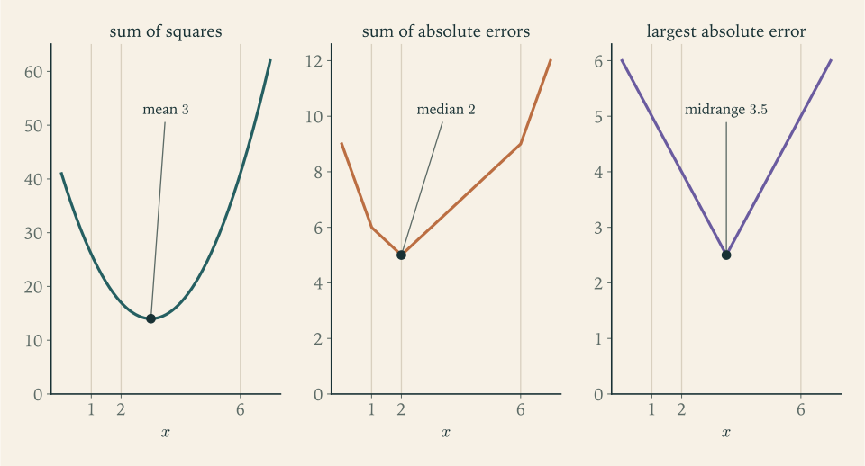
Figure 1.1 carries a warning for later chapters. Only the first objective can be minimized by setting a derivative to zero. The other two are minimized at points where the derivative does not exist, and they will need either a reformulation, as above, or the nonsmooth tools of Chapter 9.
Common mistake. Applying a transformation outside the range where it is monotone. Consider minimizing \(x\) subject to \(-2\le x\le 1\) . The minimizer is \(x=-2\) . Replacing the objective by \(x^{2}\) “because squaring preserves order” gives a problem whose minimizer is \(x=0\) . Squaring is increasing only on nonnegative numbers, and here the objective takes negative values. The same error occurs with constraints: \(x\ge 1\) and \(x^{2}\ge 1\) are not the same condition, because the second also admits \(x\le -1\) . Before transforming, write down the set of values the transformed quantity can take on the feasible set and check monotonicity there.
1.4 Level sets meeting a feasible region
Feasible sets in this book are built from a few geometric pieces. For a nonzero vector \(a\in\mathbb R^n\) and a number \(\beta\) , the set \(\{x:a^{\top}x=\beta\}\) is a hyperplane with normal vector \(a\) , and \(\{x:a^{\top}x\le\beta\}\) is a closed halfspace. A polyhedron is an intersection of finitely many halfspaces and hyperplanes, \(\{x:Ax\le b,\ Cx=d\}\) ; the workshop’s quadrilateral is one. The closed ball of radius \(r\) about a centre \(x_c\) is \(\{x:\lVert x-x_c\rVert\le r\}\) .
For the objective we use level sets \(\{x:f_0(x)=\gamma\}\)
and sublevel sets \(\{x:f_0(x)\le\gamma\}\)
. Recall from multivariable calculus that if \(f_0\)
is differentiable at \(x\)
and \(\nabla f_0(x)\ne 0\)
, then the gradient is perpendicular to the level set through \(x\)
and points in the direction in which \(f_0\)
increases fastest; the rate of change of \(f_0\)
at \(x\)
in a unit direction \(d\)
is \(\nabla f_0(x)^{\top}d\)
(math.multivariable-calculus.gradient). Consequently any direction \(d\)
with \(\nabla f_0(x)^{\top}d<0\)
is a direction of decrease.
These two families of sets give a picture of constrained minimization that is worth carrying in your head. Draw the feasible set. Draw the level sets of the objective, and imagine lowering the level \(\gamma\) . The optimal value is the smallest \(\gamma\) whose level set still touches the feasible set, and the optimal points are the points of contact. If the contact happens in the interior of the feasible set, the constraints play no role locally and the point must be an unconstrained local minimizer of \(f_0\) . If the contact happens on the boundary, the objective would decrease further if only the constraints allowed it, and the gradient of the objective is generally not zero there.
Example 1.5: A linear objective on a disc
Minimize \(x_1+x_2\) subject to \(x_1^2+x_2^2\le 2\) . The feasible set is a closed disc of radius \(\sqrt 2\) , so it is compact and Theorem 1.4 guarantees a minimizer. The level sets of the objective are the parallel lines \(x_1+x_2=\gamma\) , with normal vector \((1,1)\) . Lowering \(\gamma\) slides the line in the direction \(-(1,1)\) . The last line to touch the disc is tangent to the circle at the boundary point in that direction, namely
The picture can be turned into a proof with the Cauchy–Schwarz inequality: for every feasible \(x\) ,
and \(x=(-1,-1)\) is feasible with objective value \(-2\) , so it is optimal. Notice that the gradient of the objective at the solution is \((1,1)\) , not zero, and that it is a negative multiple of the gradient \((2x_1,2x_2)=(-2,-2)\) of the active constraint function. That alignment of gradients at a boundary solution is not an accident; it is the first appearance of the multiplier conditions of Chapter 6.
Common mistake. Solving the unconstrained derivative equation and ignoring the constraints. To minimize \((x-2)^2\) subject to \(0\le x\le 1\) , setting the derivative \(2(x-2)\) to zero gives \(x=2\) , which is not feasible. The correct minimizer is the feasible point nearest to \(2\) , namely \(x=1\) , where the derivative equals \(-2\) and the constraint \(x\le 1\) is active. A zero derivative characterizes minimizers only at points where every small move is allowed. Always write the variables, the domain, the objective, and every constraint before differentiating, and check any stationary point for feasibility.
1.5 Local and global, continuous and discrete
Definition 1.3 distinguishes local minimizers from global ones. Calculus detects local behaviour; the question asked is nearly always global. The next example shows both phenomena that separate them: an interior stationary point that is only locally best, and a boundary point that is globally best without being stationary.
Example 1.6: A local minimizer that loses to the boundary
Minimize \(f(x)=x^3-3x\) subject to \(-3\le x\le 3\) . The feasible set is compact, so a global minimizer exists. The derivative \(f'(x)=3x^2-3\) vanishes at \(x=1\) and \(x=-1\) . Since \(f''(1)=6>0\) , the point \(x=1\) is a local minimizer, with \(f(1)=-2\) ; since \(f''(-1)=-6<0\) , the point \(x=-1\) is a local maximizer, with \(f(-1)=2\) . At the endpoints, \(f(-3)=-18\) and \(f(3)=18\) .
Comparing the candidates, the global minimizer is the endpoint \(x^\star=-3\) with \(p^\star=-18\) , where \(f'(-3)=24\ne 0\) . The interior local minimizer \(x=1\) is feasible, stationary, and has positive curvature, and it is worse than the optimum by \(16\) . A method that only looks for points with zero derivative would report it and stop.
The remedy for the gap between local and global is structure. The next chapter introduces convexity, the property under which every local minimizer is global, so that local tests become conclusive.
The word continuous in the title of this book refers to the feasible set: the variables range over a region of \(\mathbb R^n\)
in which one can move by arbitrarily small steps, so that derivatives carry information about nearby feasible points. Consider choosing portfolio weights \(x\in\mathbb R^n\)
to minimize the variance \(x^{\top}\Sigma x\)
subject to the budget constraint \(\mathbf 1^{\top}x=1\)
, where \(\Sigma\)
is a covariance matrix and \(\mathbf 1\)
is the vector of ones. That is a continuous problem with a smooth objective and one linear equality constraint. Add the requirement that each asset is either held at a fixed weight or not at all, so that \(x_i\)
may take only two values, and the feasible set breaks into isolated pieces. Small moves are no longer available and the calculus-based theory stops applying directly. Problems with integrality belong to Discrete Optimization, where formulations with integer variables are developed (math.discrete-optimization.integer-formulations); what the present course contributes to them is the relaxation bound of Proposition 1.8.
Within continuous optimization, problems are classified by the kind of functions involved, because the available guarantees depend on that classification. A linear program has affine objective and constraint functions, as in Example 1.1. A quadratic program has a quadratic objective and affine constraints. A convex program has convex objective and inequality constraint functions and affine equality constraints; linear programs and many quadratic programs are special cases. Everything else is a general nonlinear program, for which one can usually certify only local optimality. The classification is not cosmetic. For a convex program, a point satisfying the optimality conditions of Chapter 6 is a global solution and comes with a certificate; for a general nonlinear program, the same conditions identify candidates and nothing more.
The questions this chapter leaves open set the agenda. When is a local minimizer automatically global? Chapter 2 answers with convexity. How does one recognise a minimizer when no constraint is active? Chapter 3 answers with first- and second-order conditions. Why is the workshop’s optimum at a corner, and how does one find the right corner without listing them all? That is Chapter 4.
Exercises
-
Write the problem “maximize \(x_1x_2\) subject to \(x_1+2x_2\le 8\) , \(x_1\ge 0\) , \(x_2\ge 0\) ” in the standard form of Definition 1.1, naming \(f_0\) , every \(f_i\) , and the numbers \(m\) and \(p\) ; then find \(p^\star\) for the standard-form problem.
Answer
Standard form: minimize \(f_0(x)=-x_1x_2\) subject to \(f_1(x)=x_1+2x_2-8\le 0\) , \(f_2(x)=-x_1\le 0\) , \(f_3(x)=-x_2\le 0\) , so \(m=3\) and \(p=0\) . The product is largest on the line \(x_1+2x_2=8\) ; substituting \(x_1=8-2x_2\) gives \((8-2x_2)x_2\) , maximal at \(x_2=2\) , \(x_1=4\) . Hence \(p^\star=-8\) .
-
For each problem decide whether it is infeasible, unbounded below, has an attained optimal value, or has a finite value that is not attained, and give \(p^\star\) : (a) minimize \(1/x\) over \(x\ge 1\) ; (b) minimize \(x^2-4x\) over \(x\ge 0\) ; (c) minimize \(-x_1\) subject to \(x_1+x_2\le 1\) ; (d) minimize \(x\) subject to \(x^2\le -1\) .
Answer
(a) \(p^\star=0\) , finite but not attained, since \(1/x>0\) and \(1/x\to 0\) . (b) \(p^\star=-4\) , attained at \(x=2\) . (c) Unbounded below, \(p^\star=-\infty\) : take \(x=(s,-s)\) with \(s\to\infty\) . (d) Infeasible, \(p^\star=+\infty\) .
-
Feed A costs 2 per kilogram and supplies 3 units of protein and 1 unit of fat per kilogram; feed B costs 3 per kilogram and supplies 1 unit of protein and 2 units of fat. A ration needs at least 9 units of protein and 8 units of fat. Formulate the cheapest ration as a problem in standard form with units for each variable, then evaluate the cost at each corner of the feasible region and identify the cheapest corner.
Solution
Let \(a\) and \(b\) be the kilograms of feed A and feed B in the ration. The cost is \(2a+3b\) . Protein supplied is \(3a+b\) units and must be at least \(9\) ; fat supplied is \(a+2b\) units and must be at least \(8\) . In standard form:
\[ \begin{aligned} \text{minimize}\quad & 2a+3b\\ \text{subject to}\quad & 9-3a-b\le 0,\quad 8-a-2b\le 0,\quad -a\le 0,\quad -b\le 0. \end{aligned} \]The feasible region is the part of the first quadrant above both lines \(3a+b=9\) and \(a+2b=8\) . It is unbounded, but the cost is coercive on it because both coefficients are positive, so a minimizer exists by Theorem 1.4. The corners are where two constraints are active. On the \(b\) -axis the protein line gives \((0,9)\) , which satisfies the fat constraint since \(18\ge 8\) ; its cost is \(27\) . On the \(a\) -axis the fat line gives \((8,0)\) , which satisfies the protein constraint since \(24\ge 9\) ; its cost is \(16\) . The two lines cross where \(3a+b=9\) and \(a+2b=8\) ; eliminating \(b\) gives \(5a=10\) , so \((a,b)=(2,3)\) with cost \(4+9=13\) . The cheapest corner is \((2,3)\) with cost \(13\) . Both nutrient constraints are active there and both sign constraints are inactive.
-
Let \(\mathcal F\subseteq\mathbb R^n\) be nonempty and closed and let \(f_0\) be continuous and coercive on \(\mathcal F\) . Prove that the optimal set is nonempty, closed, and bounded.
Solution
Fix any \(\hat x\in\mathcal F\) and put \(\gamma=f_0(\hat x)\) . The sublevel set \(S_\gamma=\{x\in\mathcal F:f_0(x)\le\gamma\}\) contains \(\hat x\) . It is bounded: otherwise it would contain points \(x_k\) with \(\lVert x_k\rVert\to\infty\) and \(f_0(x_k)\le\gamma\) , contradicting coercivity. Theorem 1.4 now gives a global minimizer, so the optimal set \(X^\star\) is nonempty.
Write \(p^\star\) for the optimal value, which is finite since it is attained. Then \(X^\star=\{x\in\mathcal F:f_0(x)\le p^\star\}=S_{p^\star}\) . It is bounded because \(S_{p^\star}\subseteq S_\gamma\) . It is closed by the argument in the proof of Theorem 1.4: a limit of points of \(\mathcal F\) lies in \(\mathcal F\) because \(\mathcal F\) is closed, and a limit of points with \(f_0\le p^\star\) has \(f_0\le p^\star\) because \(f_0\) is continuous. So \(X^\star\) is nonempty, closed, and bounded, that is, a nonempty compact set.
-
Decide whether each function is coercive on \(\mathbb R^2\) , justifying each answer with an inequality or with a direction along which the function stays bounded: (a) \(x_1^2+x_2^2-x_1x_2\) ; (b) \(x_1^2-2x_1x_2+x_2^2\) ; (c) \(x_1^4+x_2^4-4x_1x_2\) .
Hint
(a) Use \(x_1x_2\le\tfrac12(x_1^2+x_2^2)\) to bound the function below by \(\tfrac12\lVert x\rVert^2\) ; coercive. (b) The function is \((x_1-x_2)^2\) ; look along \(x_1=x_2\) ; not coercive. (c) Use \(x_1^4+x_2^4\ge\tfrac12(x_1^2+x_2^2)^2\) and \(4x_1x_2\le 2\lVert x\rVert^2\) to get the lower bound \(\tfrac12\lVert x\rVert^4-2\lVert x\rVert^2\) ; coercive.
-
Suppose \(\varphi\) is nondecreasing on the range of \(f_0\) but not strictly increasing. Prove that every minimizer of \(f_0\) over \(\mathcal F\) is still a minimizer of \(\varphi\circ f_0\) , and show by an example that \(\varphi\circ f_0\) can have minimizers that are not minimizers of \(f_0\) .
Solution
Let \(x^\star\) minimize \(f_0\) over \(\mathcal F\) , so \(f_0(x^\star)\le f_0(x)\) for every \(x\in\mathcal F\) . A nondecreasing \(\varphi\) preserves weak inequalities: \(s\le t\) implies \(\varphi(s)\le\varphi(t)\) . Applying this with \(s=f_0(x^\star)\) and \(t=f_0(x)\) gives \(\varphi(f_0(x^\star))\le\varphi(f_0(x))\) for every \(x\in\mathcal F\) , so \(x^\star\) minimizes \(\varphi\circ f_0\) .
The converse fails because a nondecreasing function can be flat. Take \(\mathcal F=[0,2]\) , \(f_0(x)=x\) , and \(\varphi(t)=\max\{t,1\}\) . The only minimizer of \(f_0\) is \(x=0\) . But \(\varphi(f_0(x))=1\) for every \(x\in[0,1]\) , and \(\varphi(f_0(x))=x>1\) for \(x>1\) , so every point of \([0,1]\) minimizes \(\varphi\circ f_0\) . The points of \((0,1]\) are minimizers of the transformed problem and not of the original one. Strict monotonicity is what rules this out: it makes the implication between the two orderings run in both directions.
-
A student replaces “minimize \(x\) subject to \(-2\le x\le 1\) ” by “minimize \(x^2\) subject to \(-2\le x\le 1\) ”, arguing that squaring is monotone. Find the minimizers of both problems and name the hypothesis of Proposition 1.7 that fails.
Answer
The first problem has the single minimizer \(x=-2\) with value \(-2\) ; the second has the single minimizer \(x=0\) with value \(0\) . The range of the objective \(x\) on the feasible set is \([-2,1]\) , and \(t\mapsto t^2\) is not strictly increasing on any interval containing negative numbers, so the monotonicity hypothesis of Proposition 1.7 fails.
-
Rewrite “minimize \(\max\{2x+1,\ -x+4,\ \tfrac12 x+2\}\) over \(x\in\mathbb R\) ” as a linear program in the variables \((x,t)\) , and solve it by finding where the active pieces cross.
Solution
Introduce \(t\) and require each piece to lie below it. The linear program is
\[ \begin{aligned} \text{minimize}\quad & t\\ \text{subject to}\quad & 2x+1-t\le 0,\quad -x+4-t\le 0,\quad \tfrac12x+2-t\le 0 . \end{aligned} \]For fixed \(x\) the smallest feasible \(t\) is the maximum of the three pieces, so this is the epigraph form of the original problem. The piece \(2x+1\) is increasing and the piece \(-x+4\) is decreasing, and they cross where \(2x+1=-x+4\) , that is, at \(x=1\) , where both equal \(3\) . The third piece equals \(2.5\) there, which is smaller, so it is inactive. To the left of \(x=1\) the decreasing piece exceeds \(3\) ; to the right the increasing piece exceeds \(3\) . Hence the maximum of the three pieces is at least \(3\) everywhere and equals \(3\) only at \(x=1\) . The solution is \((x,t)=(1,3)\) , with the first two constraints active.
-
Convert the constraints \(x_1+x_2\le 4\) and \(2x_1+x_2\le 5\) of Example 1.1 into equations with nonnegative slack variables \(s_1,s_2\) , and give the slack values at each of the four corners of the feasible set.
Answer
The equations are \(x_1+x_2+s_1=4\) and \(2x_1+x_2+s_2=5\) with \(s_1,s_2\ge 0\) . At \((0,0)\) : \(s=(4,5)\) . At \((2.5,0)\) : \(s=(1.5,0)\) . At \((1,3)\) : \(s=(0,0)\) . At \((0,4)\) : \(s=(0,1)\) . A slack is zero exactly when its constraint is active.
-
Eliminate the equality constraint from “minimize \(x_1^2+2x_2^2\) subject to \(x_1+x_2=3\) ” by substituting \(x_2=3-x_1\) , solve the one-variable problem, and report the minimizer and the optimal value of the original problem.
Answer
The reduced objective is \(x_1^2+2(3-x_1)^2\) with derivative \(6x_1-12\) , so \(x_1=2\) , \(x_2=1\) , and the optimal value is \(4+2=6\) . The reduced objective is a coercive quadratic in \(x_1\) with positive leading coefficient, so the stationary point is its global minimizer.
-
For the data \(b=(0,1,5,10)\) find the minimizer of \(\sum_i(x-b_i)^2\) , all minimizers of \(\sum_i\lvert x-b_i\rvert\) , and the minimizer of \(\max_i\lvert x-b_i\rvert\) ; explain why the second problem has more than one solution.
Solution
Squares. The derivative of \(\sum_i(x-b_i)^2\) is \(2\sum_i(x-b_i)=8x-32\) , which vanishes at the mean \(x=4\) . The objective is a parabola opening upward, so this is the unique minimizer; the value is \(16+9+1+36=62\) .
Absolute values. The objective is piecewise linear. Its slope on an interval between data points equals the number of data points to the left minus the number to the right. Left of \(0\) the slope is \(-4\) ; on \((0,1)\) it is \(-2\) ; on \((1,5)\) it is \(0\) ; on \((5,10)\) it is \(+2\) ; right of \(10\) it is \(+4\) . So the function decreases up to \(x=1\) , is constant on \([1,5]\) , and increases after \(5\) . Every \(x\in[1,5]\) is a minimizer, with value \(x+(x-1)+(5-x)+(10-x)=14\) . The solution is not unique because with an even number of data points there is an interval on which as many points lie to the left as to the right, and there the slope is zero.
Largest error. Only the extreme observations matter: \(\max_i\lvert x-b_i\rvert=\max\{x-0,\,10-x\}\) for \(0\le x\le 10\) , which is minimized where the two are equal, at the midrange \(x=5\) , with value \(5\) .
-
Minimize \(2x_1+x_2\) over the disc \(x_1^2+x_2^2\le 5\) using the level-line picture of Section 1.4, then confirm the answer with the Cauchy–Schwarz inequality.
Answer
The level lines have normal \((2,1)\) ; the last one to touch the disc of radius \(\sqrt5\) does so at \(x^\star=-\sqrt5\,(2,1)/\sqrt5=(-2,-1)\) , with \(p^\star=-5\) . Cauchy–Schwarz: \(2x_1+x_2\ge-\lVert(2,1)\rVert\lVert x\rVert\ge-\sqrt5\cdot\sqrt5=-5\) , with equality at \((-2,-1)\) .
-
Let \(\mathcal F\) be the feasible set of Example 1.1. Show that for the objective \(-2x_1-x_2\) the optimal set is an entire edge of \(\mathcal F\) and say which one, and find the optimal point for the objective \(x_1+x_2\) .
Hint
The level lines of \(-2x_1-x_2\) are parallel to the finishing constraint \(2x_1+x_2=5\) . Evaluate the objective at the four corners and notice a tie between \((2.5,0)\) and \((1,3)\) ; every point of the segment joining them has the same value \(-5\) . For \(x_1+x_2\) , both coefficients are positive and the variables are nonnegative.
-
The problem “minimize \((x_1-3)^2+(x_2-2)^2\) subject to \(x_1+x_2\le 4\) with \(x_1,x_2\) integers” has a continuous relaxation obtained by dropping integrality, whose minimizer is \((2.5,1.5)\) with value \(0.5\) . Say what Proposition 1.8 tells you about the integer problem, and find the integer optimum by examining nearby integer points.
Solution
The integer feasible set is contained in the continuous one, so Proposition 1.8 gives a lower bound: the integer optimal value is at least \(0.5\) . The relaxed minimizer \((2.5,1.5)\) is not an integer point, so the second half of the proposition does not apply and the bound need not be tight.
To find the integer optimum, note that the objective is the squared distance to \((3,2)\) , and \((3,2)\) itself violates \(x_1+x_2\le 4\) . An integer point with objective value below \(1\) would have to be at distance less than \(1\) from \((3,2)\) , and the only integer point that close is \((3,2)\) itself. So the integer optimal value is at least \(1\) . The points \((2,2)\) and \((3,1)\) are feasible, since their coordinates sum to \(4\) , and each has objective value \(1\) . Therefore the integer optimal value is \(1\) , attained at \((2,2)\) and at \((3,1)\) . The relaxation bound \(0.5\le 1\) holds with a gap of \(0.5\) , and rounding the relaxed solution to the nearest integers does not by itself tell you which rounding is feasible.
-
Find all local minimizers and all global minimizers of \(f(x)=x^2(x-2)^2\) on the interval \(-1\le x\le 3\) , and describe the optimal set.
Answer
\(f\ge 0\) and \(f(x)=0\) exactly at \(x=0\) and \(x=2\) , both in the interval, so the optimal set is \(\{0,2\}\) and \(p^\star=0\) . These are also the only local minimizers: \(f'(x)=4x(x-1)(x-2)\) vanishes at \(0,1,2\) , the point \(x=1\) is a local maximizer with \(f(1)=1\) , and the endpoints have \(f(-1)=f(3)=9\) with the function decreasing as one moves inward.
-
Prove that the feasible set of Definition 1.1 is closed whenever \(\mathcal D=\mathbb R^n\) and every \(f_i\) and \(h_j\) is continuous, and give an example in which replacing \(f_1(x)\le 0\) by the strict inequality \(f_1(x)<0\) destroys attainment.
Hint
For closedness, write \(\mathcal F\) as an intersection of the sets \(\{x:f_i(x)\le 0\}\) and \(\{x:h_j(x)=0\}\) and show each is closed using sequences, as in the proof of Theorem 1.4; an intersection of closed sets is closed. For the example, compare minimizing \(x\) subject to \(-x\le 0\) with minimizing \(x\) subject to \(-x<0\) .
-
Formulate “find the point of the plane \(x_1+2x_2+2x_3=9\) nearest to the origin” as a problem in standard form, explain why a minimizer exists, and find it using the fact, from the level-set picture, that the minimizer is a multiple of the normal vector \((1,2,2)\) .
Solution
In standard form: minimize \(f_0(x)=x_1^2+x_2^2+x_3^2\) subject to \(h_1(x)=x_1+2x_2+2x_3-9=0\) . By Proposition 1.7 minimizing the squared distance is equivalent to minimizing the distance, since distances are nonnegative. A minimizer exists by Theorem 1.4: the plane is closed and nonempty, and \(f_0=\lVert x\rVert^2\) is continuous and coercive.
The level sets of \(f_0\) are spheres about the origin. The smallest sphere that touches the plane is tangent to it, and at the point of tangency the radius is perpendicular to the plane, so the minimizer is \(x=s(1,2,2)\) for some scalar \(s\) . Feasibility requires \(s(1+4+4)=9\) , so \(s=1\) and \(x^\star=(1,2,2)\) , at distance \(\lVert x^\star\rVert=3\) from the origin.
To confirm without the picture, take any feasible \(x\) and write \(x=x^\star+d\) . Feasibility of both points gives \((1,2,2)^{\top}d=0\) , that is, \(x^{\star\top}d=0\) . Then \(\lVert x\rVert^2=\lVert x^\star\rVert^2+2x^{\star\top}d+\lVert d\rVert^2=9+\lVert d\rVert^2\ge 9\) , with equality only for \(d=0\) .
-
Explain what is wrong with this argument and what the true situation is: “The function \(e^{-x}\) is continuous and bounded below by \(0\) on the closed set \(x\ge 0\) , so by Theorem 1.4 it attains its minimum there.”
Answer
Theorem 1.4 requires a nonempty bounded sublevel set, and that was not checked. Here every sublevel set \(\{x\ge 0:e^{-x}\le\gamma\}\) with \(0<\gamma\le 1\) is the unbounded interval \([-\log\gamma,\infty)\) . Being bounded below is not the same as attaining the bound: \(p^\star=0\) and it is not attained, because \(e^{-x}>0\) for every \(x\) .