Two obstacles stop the gradient method of Chapter 7 from being applied to many problems of practical interest. The first is a constraint: a gradient step from a feasible point may land outside the feasible set, and at a constrained solution the gradient is not zero, so neither the iteration nor its stopping test survives. The second is a kink: for the objective \(\tfrac12\lVert Ax-b\rVert^2+\lambda\lVert x\rVert_1\) , which is used to find sparse solutions of linear systems, the gradient does not exist at exactly the points one hopes to reach, those with zero components, and Exercise 7.10 showed the gradient iteration cycling forever on \(\lvert x\rvert\) .

Both obstacles yield to one idea. Split the problem into a smooth part, handled by a gradient step, and a simple part, a constraint set or a nonsmooth penalty, handled exactly by a small auxiliary minimization that has a closed-form solution. For a constraint the auxiliary problem is a projection; for a penalty it is the proximal operator. The resulting methods cost barely more per iteration than the gradient method and inherit its convergence rates, with a proof that repeats that of Theorem 7.6 after one inequality has been replaced.

9.1 Projection onto a closed convex set

The gradient vanishes at an unconstrained minimizer. Over a convex set the right condition is an inequality.

The condition says that no feasible direction is a descent direction. In the interior of \(C\) every direction is feasible and the condition forces \(\nabla f(x^\star)=0\) ; on the boundary it allows a nonzero gradient provided it points, loosely speaking, into the set.

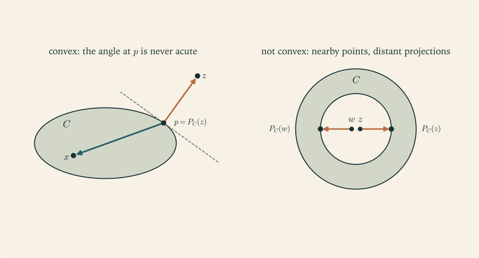
Geometrically, the vector from \(p\) to \(z\) and the vector from \(p\) to any point \(x\) of \(C\) make an angle of at least ninety degrees. When \(C\) is a subspace, both \(x-p\) and its negative are admissible, the inequality becomes an equality, and the theorem reduces to the orthogonal projection of linear algebra, where the residual \(z-p\) is perpendicular to the subspace (math.linear-algebra.projection-as-best-approximation). In infinite-dimensional Hilbert spaces the same statement is the projection theorem of functional analysis (math.functional-analysis.hilbert-projection-theorem).

The corollary is the simplest case of the separating hyperplane theorem that Chapter 6 quoted as Theorem 6.5: the hyperplane through \(p\) with normal \(z-p\) has \(C\) on one side and \(z\) strictly on the other.

Example 9.2: What goes wrong without convexity

Let \(C=\{x\in\mathbb R^2:1\le\lVert x\rVert\le1.7\}\) , a ring. It is closed and not convex. For a point \(z\) inside the hole, with \(0<\lVert z\rVert<1\) , the nearest point of \(C\) is \(z/\lVert z\rVert\) on the inner circle. For \(z=0\) every point of the inner circle is at distance \(1\) , so the nearest point is not unique. And the map is violently expansive near the centre: the points \(z=(0.12,0)\) and \(w=(-0.12,0)\) are \(0.24\) apart, while their nearest points \((1,0)\) and \((-1,0)\) are \(2\) apart.

Every part of Theorem 9.2 used convexity: uniqueness through strict convexity over a convex set, and the angle condition through Lemma 9.1. Without it, “the projection” may not be a function, and the analysis below does not apply.

9.2 The projected gradient method

To minimize a convex differentiable \(f\) over a closed convex set \(C\) , take a gradient step and project the result back:

The first question to ask of any iteration is whether the solutions are exactly the points it leaves alone.

The proposition holds for every step size, which shows that the fixed-point property is about the geometry of the solution, not about the algorithm’s parameters.

9.3 Subgradients and the proximal operator

To handle a kink we need a substitute for the gradient at a point of nondifferentiability. For convex functions the tangent inequality of Theorem 2.5 supplies one: keep every vector that satisfies it.

The value \(+\infty\) is allowed so that one definition covers the two kinds of function used in this chapter: convex functions that are finite everywhere, and the indicator \(\iota_C\) of a nonempty closed convex set \(C\) , which is \(0\) on \(C\) and \(+\infty\) outside. For an indicator and a point \(x\in C\) , the inequality is automatic at every \(y\notin C\) , where the left side is \(+\infty\) , and at \(y\in C\) it reads \(0\ge v^{\top}(y-x)\) . So

the set of vectors that make an angle of at least ninety degrees with every direction leading from \(x\) into \(C\) .

Where \(g\) is differentiable, Theorem 2.5 shows that \(\nabla g(x)\) is a subgradient, and it is the only one. At a kink there are several. For \(g(x)=\lvert x\rvert\) on \(\mathbb R\) : at \(x>0\) the subdifferential is \(\{1\}\) ; at \(x<0\) it is \(\{-1\}\) ; at \(x=0\) a number \(v\) is a subgradient exactly when \(\lvert y\rvert\ge vy\) for all \(y\) , that is, when \(-1\le v\le1\) , so \(\partial g(0)=[-1,1]\) . For \(\lVert x\rVert_1\) on \(\mathbb R^n\) the subdifferential is the product of these sets coordinate by coordinate. We use without proof the fact that a convex function finite on all of \(\mathbb R^n\) is continuous and has at least one subgradient at every point.

The definition makes the optimality condition a tautology, and a useful one: \(x^\star\) minimizes \(g\) over \(\mathbb R^n\) if and only if \(0\in\partial g(x^\star)\) , since \(v=0\) in the defining inequality reads \(g(y)\ge g(x^\star)\) . For \(\lvert x\rvert\) this correctly identifies \(0\) as the minimizer, the point at which no derivative exists.

The proximal operator returns a point that compromises between making \(g\) small and staying near \(z\) ; the parameter \(\alpha\) sets the exchange rate. The minimizer exists and is unique: the objective is continuous, it is strongly convex because it is a convex function plus \(\tfrac1{2\alpha}\lVert x-z\rVert^2\) , and it is coercive because \(g\) is bounded below by an affine function, namely any of its tangent supports.

For a differentiable \(g\) the theorem reads \(p=z-\alpha\nabla g(p)\) : a gradient step in which the gradient is evaluated at the destination and not at the origin, sometimes called an implicit step.

The operator shrinks every coordinate toward zero by the amount \(\alpha\tau\) and sets to exactly zero those that would cross it. This is the mechanism by which the \(\ell_1\) penalty produces sparse solutions: a whole interval of inputs is mapped to zero, something no smooth penalty does.

9.4 The proximal gradient method

Consider now the composite problem

where \(f\) is convex and \(L\) -smooth and \(g\) is convex with an inexpensive proximal operator: either a finite convex function, or the indicator of a nonempty closed convex set.

When \(g=0\) the proximal operator is the identity, the method is the gradient method, and \(G_\alpha=\nabla f\) . When \(g\) is an indicator, the method is the projected gradient method. When \(g=\tau\lVert\cdot\rVert_1\) it is a gradient step followed by soft thresholding. The gradient mapping plays the role that the gradient played in Chapter 7, and the next theorem shows it does so in every respect that matters.

The nonsmooth term costs nothing in the rate. Compare the subgradient method, which treats a nonsmooth convex \(F\) by stepping against an arbitrary subgradient, \(x_{i+1}=x_i-\alpha v_i\) with \(v_i\in\partial F(x_i)\) . Suppose every subgradient met has norm at most \(G\) and \(\lVert x_0-x^\star\rVert\le R\) . Expanding the square and using the subgradient inequality \(v_i^{\top}(x_i-x^\star)\ge F(x_i)-F(x^\star)\) gives \(\lVert x_{i+1}-x^\star\rVert^2\le\lVert x_i-x^\star\rVert^2-2\alpha\,(F(x_i)-F(x^\star))+\alpha^2G^2\) . Summing over \(i=0,\dots,k-1\) shows that the best of the first \(k\) values exceeds \(F(x^\star)\) by at most \((R^2+k\alpha^2G^2)/(2k\alpha)\) , which for the step \(\alpha=R/(G\sqrt k)\) equals \(RG/\sqrt k\) . It is a result of complexity theory, quoted here without proof, that no method using only function values and subgradients can improve on the order \(1/\sqrt k\) for this class of problems when the dimension exceeds \(k\) . By handling the nonsmooth term exactly through its proximal operator, the proximal gradient method achieves the \(1/k\) of the smooth case. If in addition \(f\) is \(m\) -strongly convex, the argument of Theorem 7.7 adapts to give the linear rate \((1-m/L)^k\) ; we do not repeat it. All the statements remain valid when \(L\) is replaced by any upper bound on the smoothness constant.

9.5 The gradient mapping as a certificate

At a constrained or nonsmooth solution the gradient of the smooth part is generally not zero, so \(\lVert\nabla f(x)\rVert\) cannot serve as a stopping test. Theorem 9.11(b) identifies the replacement: \(G(x)=0\) exactly at solutions, and \(\lVert G(x_k)\rVert^2\le2L\,(F(x_k)-F(x_{k+1}))\) tends to zero along the iteration. In Example 9.3 the gradient at the solution is \((0,1.5)\) while the gradient mapping is \((0,0)\) ; at the iterate \(x_2=(\tfrac49,0)\) the gradient mapping is \(3\,(x_2-x_3)=(-\tfrac19,0)\) , which correctly reports that only the first coordinate still needs to move.

For a strongly convex smooth part the mapping also bounds the distance to the solution, in the manner of Proposition 3.6, and for general convex problems one can pair it with a dual bound as in Chapter 5. The next chapter assembles such pieces into termination certificates.

Projection and proximal methods handle constraints that are simple enough to project onto. Constraints given by general inequalities \(f_i(x)\le0\) rarely are. The final chapter surveys the algorithms designed for those, and what each can honestly claim on termination.

Exercises

1. Project the point \(z=(3,-1,0.5)\) onto each of the following sets: (a) the box \([0,1]^3\) ; (b) the Euclidean ball of radius \(2\) centred at the origin; (c) the hyperplane \(x_1+x_2+x_3=1\) ; (d) the nonnegative orthant.

   Answer

   (a) Clip each coordinate: \((1,0,0.5)\) . (b) \(\lVert z\rVert=\sqrt{10.25}\approx3.2016>2\) , so the projection is \(2z/\lVert z\rVert\approx(1.874,-0.625,0.312)\) . (c) Subtract the excess along the normal: \(z-\tfrac{2.5-1}{3}(1,1,1)=(2.5,-1.5,0)\) . (d) Replace negative coordinates by zero: \((3,0,0.5)\) .

2. Prove, using the characterization in Theorem 9.2, that for \(a\ne0\) and \(a^{\top}z>\beta\) the projection of \(z\) onto the halfspace \(\{x:a^{\top}x\le\beta\}\) is \(z-\dfrac{a^{\top}z-\beta}{\lVert a\rVert^2}a\) .

   Solution

   Let \(t=(a^{\top}z-\beta)/\lVert a\rVert^2\) , which is positive by assumption, and \(p=z-ta\) . Theorem 9.2 requires two things.

   First, \(p\in C\) : \(a^{\top}p=a^{\top}z-t\lVert a\rVert^2=a^{\top}z-(a^{\top}z-\beta)=\beta\) , so \(p\) lies on the boundary hyperplane and in particular in the halfspace.

   Second, the angle condition. We have \(z-p=ta\) , so for any \(x\in C\) ,

   \[ (z-p)^{\top}(x-p)=t\,a^{\top}(x-p)=t\,(a^{\top}x-\beta)\le 0, \]

   because \(t>0\) and \(a^{\top}x\le\beta\) on \(C\) . Both conditions hold, and since the projection is unique, \(p=P_C(z)\) . When \(a^{\top}z\le\beta\) the point is already in \(C\) and is its own projection; the two cases combine into \(P_C(z)=z-\max\{a^{\top}z-\beta,0\}\,a/\lVert a\rVert^2\) . The distance from \(z\) to the halfspace is \(\lVert z-p\rVert=t\lVert a\rVert=(a^{\top}z-\beta)/\lVert a\rVert\) , the familiar formula for the distance from a point to a hyperplane.

3. The proof of Corollary 9.3 shows \(\lVert P_C(z)-P_C(w)\rVert^2\le(z-w)^{\top}(P_C(z)-P_C(w))\) . Deduce from this that \(P_C\) is continuous and that it moves no two points farther apart, and decide whether \(P_C\) can be a strict contraction when \(C\) contains more than one point.

   Hint

   Apply Cauchy–Schwarz to the right side to recover Corollary 9.3; a map with \(\lVert P(z)-P(w)\rVert\le\lVert z-w\rVert\) is continuous. It cannot be a strict contraction if \(C\) has two distinct points \(x,y\) , because \(P_C(x)=x\) and \(P_C(y)=y\) , so those two are not brought closer.

4. For the unit disc \(C\) and \(z=(3,4)\) , verify directly that \(p=(0.6,0.8)\) satisfies the inequality of Theorem 9.2 for every \(x\in C\) , using the Cauchy–Schwarz inequality.

   Solution

   Here \(p=(0.6,0.8)\) has \(\lVert p\rVert=1\) , so \(p\in C\) , and \(z-p=(2.4,3.2)=4p\) . For any \(x\) in the unit disc,

   \[ (z-p)^{\top}(x-p)=4\,p^{\top}(x-p)=4\bigl(p^{\top}x-\lVert p\rVert^2\bigr)=4\bigl(p^{\top}x-1\bigr). \]

   By the Cauchy–Schwarz inequality \(p^{\top}x\le\lVert p\rVert\,\lVert x\rVert\le1\cdot1=1\) , so the expression is at most \(0\) . This is the inequality of Theorem 9.2 for every \(x\in C\) , so \(p=P_C(z)\) . Equality holds only for \(x=p\) : every other point of the disc makes a strictly obtuse angle at \(p\) with the direction of \(z\) . The distance from \(z\) to the disc is \(\lVert z-p\rVert=4\) , which is \(\lVert z\rVert-1\) as expected.

5. To minimize \((x-2)^2\) over \(C=[0,1]\) , a student “projects the gradient”, iterating \(x^+=x-\alpha P_C(f'(x))\) . Starting from \(x=0.9\) with \(\alpha=0.1\) , show that this iteration never moves, compute what the correct projected gradient step produces, and explain the conceptual error.

   Solution

   At \(x=0.9\) the derivative is \(f'(x)=2(0.9-2)=-2.2\) . “Projecting the gradient” onto \(C=[0,1]\) clips \(-2.2\) to \(0\) , so the update is \(x^+=0.9-0.1\cdot0=0.9\) . The iterate does not move. The same happens from every \(x\in[0,1]\) , since \(f'(x)=2(x-2)<0\) there and every negative number is clipped to \(0\) . The iteration is stuck at its starting point, although the minimizer over \(C\) is \(x^\star=1\) .

   The correct projected gradient step first moves and then projects the point: \(x-\alpha f'(x)=0.9+0.22=1.12\) , and \(P_C(1.12)=1\) . One step reaches the solution, and it is a fixed point: from \(x=1\) , the tentative point is \(1+0.2=1.2\) , which projects back to \(1\) .

   The conceptual error is to apply \(P_C\) to an object of the wrong kind. The set \(C\) consists of points; it says which positions are allowed. The gradient is a direction of change, not a position, and asking whether a derivative value “lies in \([0,1]\) ” has no meaning for the problem. Feasibility is a property of the tentative point \(x-\alpha\nabla f(x)\) , so that is what must be projected. Deriving the method, as the minimization of the quadratic upper model of \(f\) over \(C\) , leaves no room for this confusion.

6. For \(f(x)=(x_1-2)^2+(x_2+1)^2\) and \(C\) the unit disc, carry out the projected gradient method with \(\alpha=1/L\) from \(x_0=(0,0)\) , show that it reaches the solution in one step, and verify the fixed-point property of Proposition 9.5 at that point.

   Answer

   \(\nabla f(x)=2(x-c)\) with \(c=(2,-1)\) , so \(L=2\) and \(\alpha=\tfrac12\) . From any \(x\) , the gradient step gives \(x-(x-c)=c\) , and \(P_C(c)=c/\lVert c\rVert=(2,-1)/\sqrt5\approx(0.894,-0.447)\) . From that point the gradient step again gives \(c\) , which projects to the same point: a fixed point, hence the solution by Proposition 9.5.

7. Compute \(\operatorname{prox}_{\alpha g}(z)\) in one variable for (a) \(g(x)=\tfrac\mu2x^2\) ; (b) \(g(x)=\mu x\) ; (c) the indicator of \([0,\infty)\) ; (d) \(g(x)=\mu\lvert x\rvert\) ; in each case use Theorem 9.8 and say which inputs are mapped to zero.

   Solution

   By Theorem 9.8, \(p=\operatorname{prox}_{\alpha g}(z)\) is characterised by \((z-p)/\alpha\in\partial g(p)\) .

   (a) \(g(x)=\tfrac\mu2x^2\) is differentiable with \(g'(p)=\mu p\) , so \(z-p=\alpha\mu p\) and \(p=z/(1+\alpha\mu)\) . Only \(z=0\) is mapped to zero.

   (b) \(g(x)=\mu x\) has \(g'=\mu\) everywhere, so \(z-p=\alpha\mu\) and \(p=z-\alpha\mu\) : a pure shift. Only \(z=\alpha\mu\) is mapped to zero.

   (c) For the indicator of \([0,\infty)\) the operator is the projection onto \([0,\infty)\) (Definition 9.7), so \(p=\max\{z,0\}\) . Every \(z\le0\) is mapped to zero.

   (d) For \(g(x)=\mu\lvert x\rvert\) , Proposition 9.9 gives soft thresholding with threshold \(\alpha\mu\) : \(p=z-\alpha\mu\) for \(z>\alpha\mu\) , \(p=z+\alpha\mu\) for \(z<-\alpha\mu\) , and \(p=0\) for \(\lvert z\rvert\le\alpha\mu\) . The whole interval \([-\alpha\mu,\alpha\mu]\) is mapped to zero.

   Comparing (b) and (d): on each side of zero the absolute value is linear, and soft thresholding is the shift of case (b) with the sign of \(z\) , stopped at zero. Comparing (a) and (d): the quadratic penalty has slope zero at the origin and never produces exact zeros, while the absolute value has slopes \(\pm\mu\) arbitrarily close to the origin and so can balance a nonzero pull \(z/\alpha\) of size up to \(\mu\) while staying at zero.

8. Apply soft thresholding with threshold \(0.4\) to the vector \((1,\,-0.4,\,0.2,\,-3)\) , and state how many coordinates of the result are zero and by how much the nonzero coordinates changed.

   Answer

   The result is \((0.6,\,0,\,0,\,-2.6)\) . Two coordinates are zero: \(-0.4\) lies exactly on the threshold and \(0.2\) inside it. Each nonzero coordinate moved toward zero by \(0.4\) .

9. For the Euclidean norm \(g(x)=\mu\lVert x\rVert\) on \(\mathbb R^n\) , show that \(\partial g(0)\) is the ball of radius \(\mu\) and that \(\partial g(x)=\{\mu x/\lVert x\rVert\}\) for \(x\ne0\) , and deduce that \(\operatorname{prox}_{\alpha g}(z)=\max\{1-\alpha\mu/\lVert z\rVert,\,0\}\,z\) .

   Solution

   Subdifferential. For \(x\ne0\) the function \(\mu\lVert x\rVert\) is differentiable with gradient \(\mu x/\lVert x\rVert\) , and at a point of differentiability the gradient is the only subgradient. At \(x=0\) , a vector \(v\) is a subgradient if and only if \(\mu\lVert y\rVert\ge v^{\top}y\) for all \(y\) . If \(\lVert v\rVert\le\mu\) this holds by Cauchy–Schwarz. If \(\lVert v\rVert>\mu\) , the choice \(y=v\) gives \(v^{\top}y=\lVert v\rVert^2>\mu\lVert v\rVert\) , violating it. So \(\partial g(0)=\{v:\lVert v\rVert\le\mu\}\) .

   Proximal operator. By Theorem 9.8 we need \((z-p)/\alpha\in\partial g(p)\) . Suppose \(p\ne0\) . Then \(z-p=\alpha\mu\,p/\lVert p\rVert\) , so \(z=\bigl(1+\alpha\mu/\lVert p\rVert\bigr)p\) : the vectors \(z\) and \(p\) are positive multiples of one another, and taking norms, \(\lVert z\rVert=\lVert p\rVert+\alpha\mu\) . This requires \(\lVert z\rVert>\alpha\mu\) , and then \(\lVert p\rVert=\lVert z\rVert-\alpha\mu\) and

   \[ p=\frac{\lVert z\rVert-\alpha\mu}{\lVert z\rVert}\,z=\Bigl(1-\frac{\alpha\mu}{\lVert z\rVert}\Bigr)z . \]

   Suppose instead \(p=0\) . Then the condition is \(z/\alpha\in\partial g(0)\) , that is, \(\lVert z\rVert\le\alpha\mu\) . The two cases are exclusive and exhaustive, and together they are the formula \(p=\max\{1-\alpha\mu/\lVert z\rVert,0\}\,z\) . The operator shortens \(z\) by \(\alpha\mu\) without changing its direction and sends every vector of length at most \(\alpha\mu\) to zero. It zeroes the whole vector at once, where the \(\ell_1\) norm zeroes coordinates one by one; in one dimension the two coincide.

10. Solve the one-variable problem “minimize \(\tfrac12(x-b)^2+\lambda\lvert x\rvert\) ” for \(\lambda\ge0\) in closed form, identify the set of \(b\) for which the solution is zero, and relate the answer to Proposition 9.9.

    Answer

    The objective is the proximal objective of \(\lambda\lvert\cdot\rvert\) with \(\alpha=1\) at \(z=b\) , so by Proposition 9.9 the solution is \(b-\lambda\) for \(b>\lambda\) , \(b+\lambda\) for \(b<-\lambda\) , and \(0\) for \(\lvert b\rvert\le\lambda\) . The solution is zero exactly when \(\lvert b\rvert\le\lambda\) .

11. For \(F(x)=\tfrac12(x_1-2)^2+\tfrac12(x_2-0.5)^2+\lvert x_1\rvert+\lvert x_2\rvert\) perform one proximal gradient step from \(x_0=(0,0)\) with \(\alpha=1\) , show that the result is the minimizer, and verify the subgradient optimality condition there.

    Solution

    The smooth part is \(f(x)=\tfrac12\lVert x-c\rVert^2\) with \(c=(2,0.5)\) , so \(\nabla f(x)=x-c\) and \(L=1\) ; the nonsmooth part is \(g(x)=\lVert x\rVert_1\) , and \(\alpha=1/L=1\) .

    From \(x_0=(0,0)\) the gradient step gives \(x_0-\nabla f(x_0)=c=(2,0.5)\) . Soft thresholding with threshold \(\alpha\tau=1\) gives

    \[ x_1=(2-1,\ 0)=(1,\ 0), \]

    since \(0.5\le1\) is set to zero.

    To show that \(x_1\) is the minimizer, check \(0\in\nabla f(x_1)+\partial\lVert x_1\rVert_1\) . Here \(\nabla f(x_1)=(1-2,\ 0-0.5)=(-1,-0.5)\) . First coordinate: \(x_1>0\) , so the subgradient of the absolute value is \(1\) , and \(-1+1=0\) . Second coordinate: the value is \(0\) , the subdifferential is \([-1,1]\) , and we need \(0.5\in[-1,1]\) , which holds. So the condition is satisfied and \((1,0)\) minimizes \(F\) , with \(F(1,0)=\tfrac12+\tfrac18+1=1.625\) . A further proximal gradient step from \((1,0)\) returns \((1,0)\) , as Theorem 9.11(b) requires. The method converged in one step because the smooth part is a multiple of \(\lVert x-c\rVert^2\) and \(\alpha=1/L\) makes its quadratic model exact, so the step solves the whole problem.

12. For \(g(x)=\max\{x,x^2\}\) on \(\mathbb R\) find \(\partial g(0)\) and \(\partial g(1)\) , and use the condition \(0\in\partial g(x)\) to locate the minimizer.

    Answer

    For \(x<0\) , \(g=x^2\) (slope tending to \(0\) at \(0\) ); for \(0<x<1\) , \(g=x\) (slope \(1\) ); for \(x>1\) , \(g=x^2\) (slope \(2\) at \(1\) ). So \(\partial g(0)=[0,1]\) and \(\partial g(1)=[1,2]\) . Since \(0\in\partial g(0)\) , the minimizer is \(x=0\) .

13. Prove that the proximal operator is nonexpansive, \(\lVert\operatorname{prox}_{\alpha g}(z)-\operatorname{prox}_{\alpha g}(w)\rVert\le\lVert z-w\rVert\) , by writing the subgradient inequality of Theorem 9.8 at both points and adding.

    Solution

    Let \(p=\operatorname{prox}_{\alpha g}(z)\) and \(q=\operatorname{prox}_{\alpha g}(w)\) . By Theorem 9.8, \((z-p)/\alpha\in\partial g(p)\) and \((w-q)/\alpha\in\partial g(q)\) . Write the subgradient inequality at \(p\) evaluated at \(q\) , and at \(q\) evaluated at \(p\) :

    \[ g(q)\ge g(p)+\tfrac1\alpha(z-p)^{\top}(q-p),\qquad g(p)\ge g(q)+\tfrac1\alpha(w-q)^{\top}(p-q). \]

    Add them. The values of \(g\) cancel, and multiplying by \(\alpha\) leaves

    \[ 0\ge(z-p)^{\top}(q-p)+(w-q)^{\top}(p-q)=\bigl((z-w)-(p-q)\bigr)^{\top}(q-p). \]

    Hence \(\lVert p-q\rVert^2\le(z-w)^{\top}(p-q)\le\lVert z-w\rVert\,\lVert p-q\rVert\) by Cauchy–Schwarz, and dividing by \(\lVert p-q\rVert\) when it is nonzero gives \(\lVert p-q\rVert\le\lVert z-w\rVert\) . The proof is word for word that of Corollary 9.3 with the angle condition replaced by the subgradient inequality, which is what one expects, since projection is the proximal operator of an indicator. The same computation shows that soft thresholding never increases the distance between two vectors.

14. For the problem of Example 9.3 compute the gradient mapping \(G_{1/3}\) at \(x=(1,1)\) and at the solution \((0.5,0)\) , and compare each with the gradient at the same point.

    Answer

    At \((1,1)\) : \(\nabla f=(2,4)\) , the step lands on \((\tfrac13,0)\) after clipping, and \(G=3\bigl((1,1)-(\tfrac13,0)\bigr)=(2,3)\) . The second component is smaller than the gradient’s because the bound absorbed part of the step. At \((0.5,0)\) : \(\nabla f=(0,1.5)\) and \(G=(0,0)\) .

15. For \(C=\{x:x\ge0\}\) show that the fixed-point condition \(x^\star=P_C(x^\star-\alpha\nabla f(x^\star))\) is equivalent to the KKT conditions of “minimize \(f(x)\) subject to \(-x\le0\) ”, namely \(x^\star\ge0\) , \(\nabla f(x^\star)\ge0\) , and \(x_i^\star\,\partial f(x^\star)/\partial x_i=0\) for every \(i\) .

    Solution

    Projection onto the nonnegative orthant acts by coordinates: \(P_C(u)_i=\max\{u_i,0\}\) . Write \(d_i=\partial f(x^\star)/\partial x_i\) . The fixed-point condition is, for every \(i\) ,

    \[ x_i^\star=\max\{x_i^\star-\alpha d_i,\ 0\}. \]

    Suppose it holds. The right side is nonnegative, so \(x_i^\star\ge0\) . If \(x_i^\star>0\) , the maximum must be attained by the first argument, so \(x_i^\star=x_i^\star-\alpha d_i\) and \(d_i=0\) . If \(x_i^\star=0\) , then \(\max\{-\alpha d_i,0\}=0\) forces \(d_i\ge0\) . In both cases \(d_i\ge0\) and \(x_i^\star d_i=0\) .

    Conversely, suppose \(x^\star\ge0\) , \(d\ge0\) , and \(x_i^\star d_i=0\) for all \(i\) . If \(x_i^\star>0\) then \(d_i=0\) and \(\max\{x_i^\star,0\}=x_i^\star\) . If \(x_i^\star=0\) then \(\max\{-\alpha d_i,0\}=0\) because \(d_i\ge0\) . So the fixed-point condition holds.

    These three conditions are the KKT conditions of the problem with constraints \(-x_i\le0\) : stationarity \(\nabla f(x^\star)-\lambda=0\) identifies the multiplier as \(\lambda=\nabla f(x^\star)\) , dual feasibility is \(d\ge0\) , primal feasibility is \(x^\star\ge0\) , and complementary slackness is \(\lambda_ix_i^\star=0\) . The projected gradient fixed point and the KKT system say the same thing, the first in a form an algorithm can iterate and test.

16. Let \(C=\{x\in\mathbb R^2:\lVert x\rVert\ge1\}\) . Describe the nearest points of \(C\) to a point \(z\) with \(\lVert z\rVert<1\) , show that the origin has infinitely many nearest points, and give two points \(z,w\) for which the nearest points are farther apart than \(z\) and \(w\) .

    Answer

    For \(0<\lVert z\rVert<1\) the unique nearest point is \(z/\lVert z\rVert\) . For \(z=0\) every point of the unit circle is at distance \(1\) . Taking \(z=(0.1,0)\) and \(w=(-0.1,0)\) , at distance \(0.2\) , the nearest points \((1,0)\) and \((-1,0)\) are at distance \(2\) .

17. In Example 9.5 the smoothness bound \(3\) was used and \(\lVert x_0-x^\star\rVert^2=0.5625\) . Find the number of iterations after which Theorem 9.11(c) guarantees \(F(x_k)-F(x^\star)\le10^{-3}\) , and compare with the error actually observed at \(k=4\) .

    Answer

    The guarantee \(\tfrac{3\cdot0.5625}{2k}\le10^{-3}\) needs \(k\ge843.75\) , so \(844\) iterations. The observed error at \(k=4\) is already about \(1.6\times10^{-3}\) : the bound is a worst case over all problems with these constants.

18. Explain how Theorem 9.11 contains Theorem 7.6 as the special case \(g=0\) , and what the theorem says when \(g\) is the indicator of a closed convex set; in each case state what \(G\) becomes.

    Hint

    With \(g=0\) the proximal operator is the identity, \(G=\nabla f\) , and part (c) is Theorem 7.6. With \(g\) an indicator, the operator is \(P_C\) , \(F=f\) on \(C\) , \(G(x)=L\bigl(x-P_C(x-\nabla f(x)/L)\bigr)\) , and part (c) is the \(1/k\) rate for the projected gradient method.

19. Use Corollary 9.4 to write down a hyperplane that separates the point \(z=(3,4)\) from the unit disc, and explain how the same corollary shows that every closed convex set is the intersection of the closed halfspaces that contain it.

    Hint

    With \(p=(0.6,0.8)\) and \(a=z-p=(2.4,3.2)\) : \(a^{\top}x\le4\) on the disc and \(a^{\top}z=20\) , so any hyperplane \(3x_1+4x_2=\gamma\) with \(5\le\gamma<25\) separates them. For the second part, a point outside \(C\) is excluded by the halfspace \(\{x:a^{\top}x\le a^{\top}p\}\) that Corollary 9.4 constructs for it, and that halfspace contains \(C\) .