A solver is given a constrained problem and, some time later, prints a point and the word “optimal”. What exactly has been established? That the iterates stopped moving? That some residual fell below a tolerance, and if so, a residual of what, measured in which units? The answer matters, because Chapters 5 and 6 showed that for convex problems there is a precise standard, a primal point and a dual point whose objective values nearly agree, and that anything short of it can be badly wrong.
The algorithms of the last three chapters need help before they can meet that standard on a general constrained problem. Projection is available only for simple sets. This chapter describes the main strategies for constraints given by equations and inequalities: Newton’s method applied to the KKT system; penalty and augmented Lagrangian methods, which move constraints into the objective; and barrier methods, which keep the iterates strictly inside the feasible region and follow a path to the solution. For each we ask the same two questions: which of the KKT conditions hold exactly at every iterate, and which hold only in the limit. The chapter, and the book, end with how to choose among methods and what to report when one of them stops.
10.1 Equality constraints: Newton on the KKT system
Consider minimizing a twice continuously differentiable convex function \(f\) subject to \(Ax=b\) , where \(A\) is \(p\times n\) with independent rows. At a feasible point \(x\) , replace \(f\) by its second-order model and ask for the best feasible step: minimize \(\nabla f(x)^{\top}d+\tfrac12d^{\top}\nabla^2f(x)d\) subject to \(A(x+d)=b\) , that is, \(Ad=0\) . This is an equality-constrained quadratic program in \(d\) , and by Theorem 4.13 its solution is characterised by the linear system
The coefficient matrix is called the KKT matrix. By Theorem 4.13(c) it is invertible whenever the Hessian is positive definite on the null space of \(A\) . The step \(d\) is the Newton step for the equality-constrained problem, and \(w\) is the multiplier estimate that comes with it. Because \(Ad=0\) , every iterate remains feasible; stationarity, \(\nabla f(x)+A^{\top}\nu=0\) , is what the iteration works to achieve. With a line search along \(d\) the method inherits the convergence behaviour described in Chapter 8, since eliminating the constraints as in Section 1.3 turns it into Newton’s method on a reduced unconstrained problem.
When the objective is quadratic the model is exact and a single solve finishes the job.
Example 10.1: Constrained least squares and its two residuals
Fit the line \(y=c_0+c_1t\) to the points \((0,1)\) , \((1,2)\) , \((2,4)\) of Example 3.5, with the added requirement that the line pass through \((1,2.5)\) : minimize \(\lVert Ax-b\rVert^2\) subject to \(c_0+c_1=2.5\) . With \(A^{\top}A=\begin{pmatrix}3&3\\3&5\end{pmatrix}\) and \(A^{\top}b=(7,10)\) , the conditions \(2A^{\top}(Ax-b)+C^{\top}\nu=0\) and \(Cx=d\) , where \(C=\begin{pmatrix}1&1\end{pmatrix}\) and \(d=2.5\) , read
Subtracting the first equation from the second gives \(4c_1=6\) , so \(c_1=1.5\) , \(c_0=1\) , and then \(\nu=14-15=-1\) .
Now verify, as one should with any computed solution. Primal residual: \(Cx-d=1+1.5-2.5=0\) . Dual residual, that is, the stationarity residual: the fitted values are \((1,2.5,4)\) , so \(Ax-b=(0,0.5,0)\) , and \(2A^{\top}(Ax-b)=(1,1)\) ; adding \(C^{\top}\nu=(-1,-1)\) gives \((0,0)\) . Both residuals vanish, and since the problem is convex, Theorem 6.3 certifies the solution. The objective is \(0.25\) , compared with \(1/6\) for the unconstrained fit: the constraint costs \(0.25-0.1667\approx0.083\) .
The two residuals are separate pieces of evidence. A point can satisfy the constraint exactly and be far from stationary, or be stationary for some multiplier and violate the constraint. A certificate for an equality-constrained problem reports both.
10.2 Penalties and augmented Lagrangians
A different strategy removes the constraints by charging for their violation. Chapter 5 priced violations linearly, with the right prices unknown. The quadratic penalty method prices them quadratically, with a single parameter \(\rho>0\) : for the problem of minimizing \(f(x)\) subject to \(h(x)=0\) , where \(h:\mathbb R^n\to\mathbb R^p\) , it minimizes
without constraints, for an increasing sequence of values of \(\rho\) .
Theorem 10.1 (convergence of the quadratic penalty method). Let \(f\) and \(h\) be continuous and suppose the constrained problem has an optimal solution. For each \(\rho\) in a sequence tending to infinity let \(x_\rho\) be a global minimizer of \(Q_\rho\) . Then every limit point of the sequence \(x_\rho\) is an optimal solution of the constrained problem.
Proof. Let \(\bar x\) be optimal for the constrained problem, so \(h(\bar x)=0\) and \(Q_\rho(\bar x)=f(\bar x)\) . Since \(x_\rho\) minimizes \(Q_\rho\) ,
Let \(\hat x\) be the limit of a subsequence of the \(x_\rho\) . Along it \(f(x_\rho)\to f(\hat x)\) , so \(f(x_\rho)\) is bounded, and the inequality gives \(\lVert h(x_\rho)\rVert^2\le\tfrac2\rho(f(\bar x)-f(x_\rho))\to0\) . By continuity \(h(\hat x)=0\) : the limit is feasible. Dropping the nonnegative penalty term from the inequality and passing to the limit gives \(f(\hat x)\le f(\bar x)\) . A feasible point with objective value no larger than the optimal value is optimal.
The method never produces a feasible point for finite \(\rho\) ; feasibility is reached only in the limit. And it pays for a large \(\rho\) with ill-conditioning, as the next example shows.
Example 10.2: The penalty method on a small quadratic program
Minimize \(x_1^2+x_2^2\) subject to \(x_1+x_2=1\) , whose solution by Example 4.6 is \((\tfrac12,\tfrac12)\) with multiplier \(\nu^\star=-1\) . The penalized objective is \(Q_\rho(x)=x_1^2+x_2^2+\tfrac\rho2(x_1+x_2-1)^2\) . By symmetry its minimizer has \(x_1=x_2=s\) , and setting the derivative \(2s+\rho(2s-1)\) to zero gives
For \(\rho=1,10,100,1000\) the minimizer has \(s=0.25,\ 0.4545,\ 0.4950,\ 0.4995\) , with violations \(-0.5,\ -0.0909,\ -0.0099,\ -0.0010\) . The product \(\rho\,(x_1+x_2-1)=-\rho/(1+\rho)\) takes the values \(-0.5,\ -0.909,\ -0.990,\ -0.999\) and tends to \(-1=\nu^\star\) : the penalty method produces multiplier estimates as a by-product.
The Hessian of \(Q_\rho\) is \(2I+\rho\,\mathbf 1\mathbf 1^{\top}\) , with eigenvalues \(2\) and \(2+2\rho\) , so its condition number is \(1+\rho\) . To get the violation down to \(10^{-3}\) requires \(\rho\approx1000\) and a condition number near \(1000\) , which by Chapter 7 makes the gradient method very slow on the penalized problem, and in finite precision degrades any method.
The cure for ill-conditioning is to combine the quadratic penalty with a linear price, so that the price, not the penalty parameter, carries the burden of enforcing the constraint.
Definition 10.2 (augmented Lagrangian, method of multipliers). For the problem of minimizing \(f(x)\) subject to \(h(x)=0\) , the augmented Lagrangian with parameter \(\rho>0\) is
The method of multipliers starts from an estimate \(\nu_0\) and repeats: let \(x_{k+1}\) minimize \(L_\rho(\cdot,\nu_k)\) ; then set \(\nu_{k+1}=\nu_k+\rho\,h(x_{k+1})\) .
The update is the one that makes the new pair stationary for the ordinary Lagrangian. Indeed the minimizer \(x_{k+1}\) satisfies \(\nabla f(x_{k+1})+\sum_j\bigl(\nu_k+\rho\,h(x_{k+1})\bigr)_j\nabla h_j(x_{k+1})=0\) , which is exactly \(\nabla_xL(x_{k+1},\nu_{k+1})=0\) . So every iterate satisfies stationarity; what converges is feasibility.
Proposition 10.3 (exactness at the right multiplier). Consider a convex problem with affine equality constraints \(h(x)=Ax-b\) , and suppose \(x^\star\) is optimal with KKT multiplier \(\nu^\star\) . Then for every \(\rho>0\) , \(x^\star\) minimizes \(L_\rho(\cdot,\nu^\star)\) .
Proof. By Theorem 6.3 and Theorem 6.2, \(x^\star\) minimizes the ordinary Lagrangian \(L(\cdot,\nu^\star)\) . For any \(x\) ,
the last equality because \(h(x^\star)=0\) .
So with the right price no large penalty is needed: any \(\rho>0\) gives the exact solution. The method of multipliers approaches that situation by improving the price at a fixed, moderate \(\rho\) .
Example 10.3: The method of multipliers on the same problem
For \(x_1^2+x_2^2\) subject to \(x_1+x_2=1\) , the augmented Lagrangian is \(x_1^2+x_2^2+\nu(x_1+x_2-1)+\tfrac\rho2(x_1+x_2-1)^2\) . Its minimizer for fixed \(\nu\) has \(x_1=x_2=s\) with \(2s+\nu+\rho(2s-1)=0\) , so
The multiplier error obeys \(\nu^++1=(\nu+1)/(1+\rho)\) : it contracts by the factor \(1/(1+\rho)\) at every step. Take \(\rho=1\) and \(\nu_0=0\) . Then
and the iterates converge to \(\nu^\star=-1\) and \(s=0.5\) with the error halving each time, while the Hessian \(2I+\mathbf 1\mathbf 1^{\top}\) keeps condition number \(2\) . With \(\rho=9\) the error would shrink tenfold per step at condition number \(10\) . Compare the pure penalty method, which needed \(\rho\approx1000\) for three correct digits.
10.3 The logarithmic barrier and the central path
For inequality constraints the difficulty is combinatorial: which constraints are active? Barrier methods avoid the question by staying strictly inside the feasible region and letting the active set emerge in the limit. Consider the convex problem
with \(f_0,\dots,f_m\) convex and twice continuously differentiable, and suppose a strictly feasible point exists. Equality constraints \(Ax=b\) can be carried along throughout with the machinery of Section 10.1; we omit them to keep the formulas short.
Definition 10.4 (logarithmic barrier, central path). The logarithmic barrier of the constraints is the function
defined on the set of strictly feasible points. For \(t>0\) , a central point \(x^\star(t)\) is a minimizer of \(t\,f_0(x)+\phi(x)\) over that set. The curve \(t\mapsto x^\star(t)\) is the central path.
The barrier is finite inside the feasible region and tends to \(+\infty\) as any constraint approaches activity, so minimizing \(tf_0+\phi\) cannot leave the interior. It is convex: \(-\log(-u)\) is convex and increasing in \(u<0\) , so each term is convex by Proposition 2.7(d). Its gradient is \(\nabla\phi(x)=\sum_i\dfrac{1}{-f_i(x)}\nabla f_i(x)\) . The parameter \(t\) sets the relative weight of the objective: for small \(t\) the barrier dominates and the central point sits deep inside the region; as \(t\) grows the objective dominates and the central point is pushed toward the boundary. The main theorem says exactly how close to optimal it is.
Theorem 10.5 (duality gap of a central point). Let \(x^\star(t)\) be a central point and define
Then \(\lambda^\star(t)\) is dual feasible, \(g(\lambda^\star(t))=f_0(x^\star(t))-m/t\) , and consequently
Proof. Write \(x=x^\star(t)\) and \(\lambda=\lambda^\star(t)\) . Since \(x\) is strictly feasible, \(-f_i(x)>0\) and so \(\lambda_i>0\) . The central point minimizes a differentiable function over an open set, so the gradient vanishes there: \(t\nabla f_0(x)+\sum_i\dfrac{1}{-f_i(x)}\nabla f_i(x)=0\) . Dividing by \(t\) ,
This says that \(x\) is a stationary point of the Lagrangian \(L(\cdot,\lambda)=f_0+\sum_i\lambda_if_i\) , which is convex because \(\lambda\ge0\) . By Theorem 3.5 it is a global minimizer, so
In particular \(g(\lambda)\) is finite, so \(\lambda\) is dual feasible, and by Theorem 5.4, \(p^\star\ge g(\lambda)=f_0(x)-m/t\) .
The proof reveals what a central point is. The pair \((x^\star(t),\lambda^\star(t))\) satisfies primal feasibility, strictly; dual feasibility, strictly; stationarity, exactly; and, in place of complementary slackness,
The central path is the set of solutions of the KKT conditions with the zero on the right of complementary slackness replaced by \(1/t\) . As \(t\to\infty\) the perturbation vanishes. And the duality gap of the pair, in the sense of Proposition 5.7, is exactly \(m/t\) : every central point comes with its own certificate.
Example 10.4: A central path in one variable
Return to minimizing \((x-2)^2\) subject to \(x\le1\) , with \(p^\star=1\) , \(x^\star=1\) , \(\lambda^\star=2\) (Example 6.1). Here \(m=1\) and the central point minimizes \(t(x-2)^2-\log(1-x)\) over \(x<1\) . Setting the derivative to zero, \(2t(x-2)+\dfrac{1}{1-x}=0\) , that is, \(2t(x-2)(x-1)=1\) , a quadratic whose root below \(1\) is
| \(t\) | \(x^\star(t)\) | \(\lambda^\star(t)\) | \(f_0(x^\star(t))-p^\star\) | bound \(1/t\) |
|---|---|---|---|---|
| \(1\) | \(0.6340\) | \(2.7321\) | \(0.8660\) | \(1\) |
| \(10\) | \(0.9523\) | \(2.0954\) | \(0.0977\) | \(0.1\) |
| \(100\) | \(0.9950\) | \(2.0100\) | \(0.00998\) | \(0.01\) |
The central points approach \(x^\star=1\) from inside, the multipliers approach \(2\) , and the suboptimality stays below \(1/t\) as Theorem 10.5 requires. One can also confirm the exact gap: with \(g(\lambda)=\lambda-\lambda^2/4\) from the Lagrangian \((x-2)^2+\lambda(x-1)\) , at \(t=1\) we get \(g(2.7321)=0.8660\) and \(f_0(x^\star(1))=1.8660\) , a difference of exactly \(1=m/t\) .
Example 10.5: The central path of the workshop
For the workshop problem in minimization form, with the four constraints \(x_1+x_2\le4\) , \(2x_1+x_2\le5\) , \(x_1\ge0\) , \(x_2\ge0\) , we have \(m=4\) and
Minimizing \(t(-3x_1-2x_2)+\phi(x)\) by Newton’s method for several values of \(t\) gives:
| \(t\) | central point | profit | dual value | gap \(4/t\) |
|---|---|---|---|---|
| near \(0\) | \((0.759,\ 1.118)\) | \(4.51\) | ||
| \(1\) | \((1.146,\ 1.976)\) | \(7.39\) | \(11.39\) | \(4\) |
| \(10\) | \((1.009,\ 2.888)\) | \(8.80\) | \(9.20\) | \(0.4\) |
| \(100\) | \((1.0001,\ 2.9899)\) | \(8.980\) | \(9.020\) | \(0.04\) |
The first row is the analytic centre of the quadrilateral, the minimizer of the barrier alone. As \(t\) grows, the central point moves to the optimal vertex \((1,3)\) , and the profit and the dual value close in on \(9\) from below and above with gap exactly \(4/t\) . At \(t=10\) the multipliers \(1/(t\cdot\text{slack})\) are \((0.970,\ 1.064,\ 0.099,\ 0.035)\) : the first two are approaching the shadow prices \((1,1)\) of Example 4.4, and the last two, belonging to the inactive sign constraints, are approaching zero. Without ever deciding which constraints are active, the method has found out.
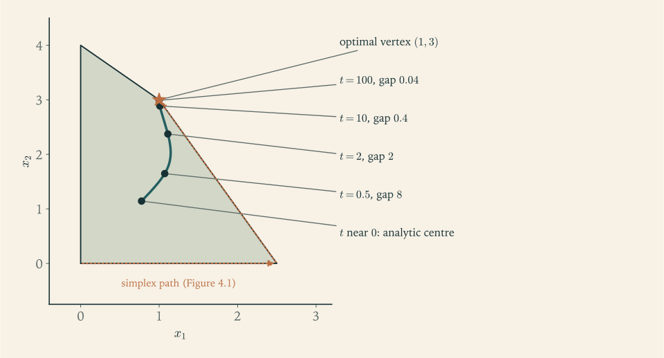
Figure 10.1 sets the two great methods for linear programs side by side. One walks along edges and stops at a vertex with an exact certificate; the other follows a smooth curve through the interior and can stop anywhere on it with a certificate of known quality.
10.4 The barrier method
Minimizing \(tf_0+\phi\) for a very large \(t\) in one go is hard, because the function changes rapidly near the boundary. Starting each minimization from the solution of the previous, easier one is efficient.
Definition 10.6 (barrier method). Given a strictly feasible \(x\) , an initial \(t>0\) , a factor \(\mu>1\) , and a tolerance \(\varepsilon>0\) , repeat: (1) centering: starting from \(x\) , compute \(x^\star(t)\) by the damped Newton method applied to \(tf_0+\phi\) , and replace \(x\) by it; (2) test: if \(m/t\le\varepsilon\) , stop; (3) increase: replace \(t\) by \(\mu t\) .
The centering step uses backtracking that also rejects trial points outside the strictly feasible set, so the iterates never cross the boundary. On termination, Theorem 10.5 guarantees \(f_0(x)-p^\star\le\varepsilon\) , up to the accuracy of the last centering. The number of outer iterations follows from the stopping rule: starting from \(t_0\) , after \(k\) increases \(t=\mu^kt_0\) , so the method stops as soon as \(\mu^kt_0\ge m/\varepsilon\) , that is, after
increases. The choice of \(\mu\) trades outer iterations against the Newton iterations needed for each centering; values between \(10\) and \(20\) work well in practice, and the total number of Newton steps is typically a few tens, almost independent of the size of the problem.
A strictly feasible starting point is required. When none is known, one is found by a preliminary Phase I problem, for example minimizing a scalar \(s\) subject to \(f_i(x)\le s\) for all \(i\) , which has an obvious strictly feasible point and whose optimal value is negative exactly when the original constraints have one.
Example 10.6: Choosing the barrier parameter
A convex problem has \(m=20\) inequality constraints and a guaranteed gap of \(10^{-6}\) is wanted. By Theorem 10.5 the final parameter must satisfy \(20/t\le10^{-6}\) , that is, \(t\ge2\times10^{7}\) . Starting from \(t_0=1\) with \(\mu=10\) , the values of \(t\) are \(1,10,100,\dots\) , and the first that is large enough is \(10^{8}\) , reached after \(8\) increases; the formula gives \(\lceil\log(2\times10^{7})/\log10\rceil=\lceil7.3\rceil=8\) . With \(\mu=20\) it gives \(\lceil7.3/1.30\rceil=6\) .
The bound \(m/t\) concerns the central point. An iterate that has not been centered accurately is not covered by it, so the certificate reported at termination should not be the nominal value \(m/t\) alone but the residuals actually measured at the final point, as Section 10.6 describes.
10.5 Active-set and sequential quadratic methods in brief
Two further families deserve mention, without analysis. Active-set methods for quadratic programs maintain a guess of the active constraints, solve the resulting equality-constrained problem by the linear system of Theorem 4.13, and revise the guess exactly as in Example 6.2: a constraint whose multiplier turns negative is dropped, and a violated constraint is added. The simplex method is the active-set method for linear programs. Such methods terminate with exact multipliers and are efficient when a good guess of the active set is available, for instance from a closely related problem solved earlier.
Sequential quadratic programming treats a general smooth nonlinear program by solving a sequence of quadratic programs, each built from a quadratic model of the Lagrangian and a linearisation of the constraints at the current point. When all constraints are equalities, the step is exactly a Newton step for the system formed by stationarity and feasibility, the generalisation of Section 10.1 to nonlinear constraints. With inequality constraints that description is only approximately right: each quadratic program also chooses an active set, and the method coincides with Newton’s method on the KKT equations of the active constraints once that set has settled. The classical local convergence result, quoted here without proof, is this. Let \(x^\star\) be a local solution with multipliers \((\lambda^\star,\nu^\star)\) at which the objective and constraint functions have Lipschitz continuous second derivatives; the gradients of the active constraints are linearly independent, as in Theorem 6.8; strict complementarity holds, meaning that every active inequality constraint has a positive multiplier; and the second-order sufficient condition holds, meaning that the Hessian of the Lagrangian in \(x\) is positive definite on the directions tangent to the active constraints. Then, if the quadratic programs use the exact Hessian of the Lagrangian and full steps are taken, the iterates and multiplier estimates converge quadratically from any starting pair sufficiently close to \((x^\star,\lambda^\star,\nu^\star)\) . For nonconvex problems the method finds KKT points, with all the caveats of Section 6.6.
10.6 What to report at termination
A solver’s status flag is not a mathematical statement. A certificate is. For a convex problem in standard form, collect the following at the final point \(x\) with multipliers \((\lambda,\nu)\) .
Definition 10.7 (KKT residuals). The primal residual is the vector of constraint violations, with components \(\max\{f_i(x),0\}\) and \(h_j(x)\) . The dual residual is the stationarity residual \(\nabla f_0(x)+\sum_i\lambda_i\nabla f_i(x)+\sum_j\nu_j\nabla h_j(x)\) , together with any violation of \(\lambda\ge0\) . The complementarity residual has components \(\lambda_if_i(x)\) . When \(x\) is feasible and \((\lambda,\nu)\) is dual feasible, the duality gap of the pair is \(f_0(x)-g(\lambda,\nu)\) .
If all three residuals are exactly zero the point is a KKT point, and for a convex problem Theorem 6.3 makes it optimal. In practice they are small, not zero, and three cautions apply.
First, each method drives a different subset of the residuals to zero exactly and the rest only in the limit, so each has a characteristic way of being wrong.
| Method | Holds at every iterate | Holds only in the limit |
|---|---|---|
| Simplex | primal feasibility, complementarity | dual feasibility |
| Newton on the KKT system | primal feasibility (from a feasible start) | stationarity |
| Quadratic penalty | stationarity for the estimate \(\rho h(x)\) | primal feasibility |
| Method of multipliers | stationarity | primal feasibility |
| Barrier | primal and dual feasibility, stationarity at central points | complementarity, at rate \(1/t\) |
| Projected or proximal gradient | primal feasibility | the gradient mapping tends to zero |
Second, residuals have units and depend on scaling. Multiplying a constraint function by \(1000\)
multiplies its violation by \(1000\)
and divides its multiplier by \(1000\)
; a tolerance of \(10^{-6}\)
on the raw residual then means something entirely different. Residuals should be reported relative to the size of the quantities involved, and the question of how rounding and conditioning limit the accuracy attainable in floating-point arithmetic belongs to numerical analysis (math.numerical-analysis.floating-point-conditioning). That theory tells you how far a computed residual can be trusted; it does not replace the residuals, the feasibility checks, and the gap, which are the optimization content of the certificate.
Third, for a problem that is not convex, small KKT residuals certify an approximate KKT point and nothing more. An honest report says so, and adds whatever further evidence is available: a second-order check, a comparison across several starting points, or a lower bound from a convex relaxation or a dual.
Example 10.7: Auditing a claimed solution
For the problem of Example 6.2, minimize \((x_1-2)^2+(x_2-1)^2\) subject to \(x_1+x_2\le2\) and \(x_2\ge0\) , a solver returns \(x=(1.4999,\ 0.5002)\) with multipliers \(\lambda=(1.0003,\ 0)\) and the message “optimal”.
Primal residual. \(f_1(x)=1.4999+0.5002-2=0.0001>0\) : the first constraint is violated by \(10^{-4}\) . \(f_2(x)=-0.5002<0\) : satisfied.
Dual residual. Stationarity gives \(\bigl(2(1.4999-2)+1.0003,\ 2(0.5002-1)+1.0003-0\bigr)=(0.0001,\ 0.0007)\) , and \(\lambda\ge0\) holds.
Complementarity. \(\lambda_1f_1(x)\approx1.0\times10^{-4}\) and \(\lambda_2f_2(x)=0\) .
The largest residual is \(7\times10^{-4}\) . The point is not feasible, so the gap of the pair is not a valid bound as it stands; but the dual value still is. From Exercise 6.17, \(g(1.0003,0)=1.0003-\tfrac12(1.0003)^2=0.499999955\) , so \(p^\star\ge0.499999955\) rigorously, by weak duality alone. The returned point has objective \(0.2501+0.2498\approx0.4999\) , slightly below \(p^\star=0.5\) , which is possible only because it is slightly infeasible. A fair report reads: residuals of order \(10^{-4}\) to \(10^{-3}\) in all three categories, optimal value \(0.5\) to about three digits. “Optimal” with no qualification claimed more than was shown.
Common mistake. Declaring a point optimal because the iterations stopped changing. Small steps show that the algorithm has stalled, not why. A gradient method with a tiny step size makes tiny steps everywhere; a penalty method with a moderate \(\rho\) settles at an infeasible point; a method on a nonconvex problem settles at a saddle. None of these is detected by the size of \(x_{k+1}-x_k\) . Report the assumptions under which the method is valid, the three residuals of Definition 10.7 with their scaling, the objective value with a lower bound or duality gap when one is available, and, for a nonconvex problem, the plain statement that the point is a candidate.
10.7 Choosing a method
The choice of algorithm follows from the structure established in the earlier chapters: whether the problem is convex, how smooth the objective is, what form the constraints take, how large \(n\) is, and what accuracy and certificate are needed.
| Problem structure | First choice | Why | Certificate at termination |
|---|---|---|---|
| Smooth, unconstrained, moderate \(n\) , Hessian available | damped Newton | quadratic local rate, insensitive to conditioning | gradient norm, Newton decrement |
| Smooth, unconstrained, large \(n\) | gradient or limited-memory BFGS | cost per step of order \(n\) | gradient norm, with \(m\) if known |
| Smooth objective, simple constraint set | projected gradient | projection in closed form | gradient mapping |
| Smooth plus a simple nonsmooth term | proximal gradient | proximal operator in closed form | gradient mapping, subgradient condition |
| Linear program | simplex or barrier | vertex structure, or path with gap \(m/t\) | primal–dual certificate |
| Linear equality constraints only | Newton on the KKT system | feasibility kept, quadratic rate | primal and dual residuals |
| Convex, general inequality constraints | barrier method | strictly feasible iterates, gap \(m/t\) | residuals and duality gap |
| Equality constraints, penalty-friendly | method of multipliers | moderate \(\rho\) , good conditioning | feasibility and stationarity residuals |
| Nonconvex | any of the above as a local method | finds stationary or KKT points | residuals, stated as a candidate |
Example 10.8: Four problems, four choices
Ridge regression with a million coefficients. Minimize \(\lVert Ax-b\rVert^2+\mu\lVert x\rVert^2\) . The objective is smooth and strongly convex with modulus at least \(2\mu\) (Exercise 3.15), unconstrained, and too large for a dense Hessian. Use a gradient method or limited-memory BFGS; stop on the gradient norm, which Proposition 3.6 converts into a bound on the error through \(m=2\mu\) .
The same regression with an \(\ell_1\) penalty. The objective is smooth plus a nonsmooth term with a closed-form proximal operator. Use the proximal gradient method of Chapter 9; stop on the gradient mapping, and verify the subgradient condition coordinate by coordinate as in Example 9.5.
A portfolio with twenty assets, a budget constraint, and no short sales. Minimize \(x^{\top}\Sigma x\) subject to \(\mathbf 1^{\top}x=1\) and \(x\ge0\) . This is a small convex quadratic program. Projected gradient is possible, because the feasible set is the simplex of Example 6.3; a barrier or active-set method gives high accuracy in a few iterations and returns multipliers that identify which assets are excluded. Report the KKT residuals and the duality gap.
A design problem with a nonconvex objective and nonlinear equality constraints. No method in this book certifies a global solution. Use sequential quadratic programming or the method of multipliers from several starting points; report the KKT residuals of each limit, check the hypotheses of Theorem 6.8 and second-order conditions where possible, and present the best point found as a candidate.
In each case the reasoning runs in the same order: classify the problem, read off which theorems apply, choose the cheapest method whose assumptions are met, and decide in advance what evidence will be accepted as a stopping certificate. That order, more than any particular algorithm, is what this book has tried to teach.
Exercises
-
Minimize \((x_1-1)^2+(x_2-2)^2+(x_3-3)^2\) subject to \(x_1+x_2+x_3=3\) by solving the KKT linear system, and report the multiplier, the primal residual, and the dual residual of your solution.
Answer
Stationarity \(2(x-c)+\nu\mathbf 1=0\) with \(c=(1,2,3)\) gives \(x=c-\tfrac\nu2\mathbf 1\) ; the constraint gives \(6-\tfrac32\nu=3\) , so \(\nu=2\) and \(x=(0,1,2)\) . Primal residual: \(0+1+2-3=0\) . Dual residual: \(2(-1,-1,-1)+2(1,1,1)=0\) .
-
For “minimize \(x^2\) subject to \(x=1\) ” find the minimizer \(x(\rho)\) of the quadratic penalty function, the constraint violation, and the multiplier estimate \(\rho\,(x(\rho)-1)\) ; determine how large \(\rho\) must be for the violation to be at most \(10^{-4}\) , and give the limit of the multiplier estimate.
Solution
The penalty function is \(Q_\rho(x)=x^2+\tfrac\rho2(x-1)^2\) , a strictly convex quadratic. Setting \(Q_\rho'(x)=2x+\rho(x-1)=0\) gives
\[ x(\rho)=\frac{\rho}{2+\rho},\qquad x(\rho)-1=-\frac{2}{2+\rho},\qquad\rho\,(x(\rho)-1)=-\frac{2\rho}{2+\rho}. \]The minimizer is infeasible for every finite \(\rho\) : it always falls short of \(1\) , because the objective \(x^2\) pulls toward \(0\) and the penalty only charges for the shortfall. The violation has size \(2/(2+\rho)\) , which is at most \(10^{-4}\) exactly when \(2+\rho\ge2\times10^{4}\) , that is, \(\rho\ge19998\) .
The multiplier estimate \(-2\rho/(2+\rho)\) tends to \(-2\) as \(\rho\to\infty\) . This is the exact multiplier: the KKT conditions of the constrained problem are \(2x+\nu=0\) and \(x=1\) , giving \(\nu^\star=-2\) . The estimate is what stationarity of \(Q_\rho\) produces automatically, since \(Q_\rho'(x)=2x+\bigl[\rho(x-1)\bigr]=0\) has the form of the stationarity condition with \(\nu\) replaced by \(\rho(x-1)\) . For example at \(\rho=18\) : \(x=0.9\) , violation \(-0.1\) , estimate \(-1.8\) .
-
Apply the method of multipliers with \(\rho=2\) and \(\nu_0=0\) to “minimize \(x^2\) subject to \(x=1\) ”: derive the formulas for \(x_{k+1}\) and \(\nu_{k+1}\) , compute three iterations, and find the factor by which the multiplier error contracts.
Solution
The augmented Lagrangian is \(L_\rho(x,\nu)=x^2+\nu(x-1)+\tfrac\rho2(x-1)^2\) . Its minimizer in \(x\) solves \(2x+\nu+\rho(x-1)=0\) , so
\[ x_{k+1}=\frac{\rho-\nu_k}{2+\rho},\qquad\nu_{k+1}=\nu_k+\rho\,(x_{k+1}-1)=\nu_k-\frac{\rho(\nu_k+2)}{2+\rho}=\frac{2\nu_k-2\rho}{2+\rho}. \]With \(\rho=2\) these become \(x_{k+1}=(2-\nu_k)/4\) and \(\nu_{k+1}=(\nu_k-2)/2\) . From \(\nu_0=0\) :
\[ x_1=0.5,\ \nu_1=-1;\qquad x_2=0.75,\ \nu_2=-1.5;\qquad x_3=0.875,\ \nu_3=-1.75 . \]The exact multiplier is \(\nu^\star=-2\) (Exercise 10.2). From the update formula, \(\nu_{k+1}+2=\dfrac{2\nu_k-2\rho+4+2\rho}{2+\rho}=\dfrac{2(\nu_k+2)}{2+\rho}\) , so the multiplier error contracts by the factor \(2/(2+\rho)\) , which is \(\tfrac12\) for \(\rho=2\) ; the errors above are \(2,1,0.5,0.25\) . The constraint violation \(x_k-1\) is \(-0.5,-0.25,-0.125\) and halves likewise. The pure penalty method with the same \(\rho=2\) would stop at \(x=0.5\) for ever; the multiplier update is what carries the iterates the rest of the way, at a fixed and harmless value of \(\rho\) .
-
For “minimize \(x\) subject to \(x\ge1\) ” compute the central point \(x^\star(t)\) , the multiplier \(\lambda^\star(t)\) , and the duality gap, and check the statement of Theorem 10.5.
Answer
With \(f_1=1-x\) the central point minimizes \(tx-\log(x-1)\) : \(t-1/(x-1)=0\) , so \(x^\star(t)=1+1/t\) and \(\lambda^\star(t)=1/(t(x-1))=1\) . The dual function is \(g(\lambda)=\inf_x\,(x+\lambda(1-x))\) , which equals \(1\) at \(\lambda=1\) . The gap is \((1+1/t)-1=1/t=m/t\) with \(m=1\) , and \(p^\star=1\) .
-
For linear constraints \(a_i^{\top}x\le b_i\) , \(i=1,\dots,m\) , derive the gradient and Hessian of the logarithmic barrier \(\phi(x)=-\sum_i\log(b_i-a_i^{\top}x)\) , and prove from the Hessian that \(\phi\) is convex.
Solution
Write \(s_i(x)=b_i-a_i^{\top}x\) for the \(i\) -th slack, positive on the domain of \(\phi\) , so that \(\phi(x)=-\sum_i\log s_i(x)\) . Since \(\nabla s_i=-a_i\) , the chain rule gives
\[ \nabla\phi(x)=-\sum_{i=1}^{m}\frac{1}{s_i(x)}\,(-a_i)=\sum_{i=1}^{m}\frac{a_i}{b_i-a_i^{\top}x}. \]Differentiating once more, the derivative of \(1/s_i\) in the direction of \(x\) is \(-(1/s_i^2)\nabla s_i=a_i/s_i^2\) , so
\[ \nabla^2\phi(x)=\sum_{i=1}^{m}\frac{a_ia_i^{\top}}{(b_i-a_i^{\top}x)^2}. \]For any direction \(d\) , \(d^{\top}\nabla^2\phi(x)d=\sum_i(a_i^{\top}d)^2/s_i(x)^2\ge0\) . So the Hessian is positive semidefinite at every point of the domain, which is an open convex set (an intersection of open halfspaces), and by Theorem 2.6 \(\phi\) is convex. The quadratic form vanishes only if \(a_i^{\top}d=0\) for every \(i\) ; so if the vectors \(a_i\) span \(\mathbb R^n\) , which holds whenever the feasible polyhedron is bounded, the Hessian is positive definite and \(\phi\) is strictly convex. The gradient formula shows the barrier’s mechanism: each constraint pushes away from its boundary along \(a_i\) with a force inversely proportional to the slack.
-
A convex problem has \(m=50\) inequality constraints and a guaranteed gap of \(10^{-4}\) is required. Find the smallest admissible final value of \(t\) , and the number of increases the barrier method needs from \(t_0=1\) with \(\mu=20\) .
Answer
\(50/t\le10^{-4}\) requires \(t\ge5\times10^{5}\) . With \(\mu=20\) and \(t_0=1\) the number of increases is \(\lceil\log(5\times10^{5})/\log20\rceil=\lceil4.38\rceil=5\) , reaching \(t=3.2\times10^{6}\) .
-
For the linear program “minimize \(x\) subject to \(0\le x\le1\) ” show that the central point is \(x^\star(t)=\bigl(t+2-\sqrt{t^2+4}\bigr)/(2t)\) , find its limits as \(t\to0\) and \(t\to\infty\) , compute the two multipliers at \(t=1\) , and verify that the duality gap is \(2/t\) .
Solution
Write the constraints as \(-x\le0\) and \(x-1\le0\) , so \(m=2\) and \(\phi(x)=-\log x-\log(1-x)\) on \(0<x<1\) . The central point minimizes \(tx-\log x-\log(1-x)\) ; setting the derivative to zero,
\[ t-\frac1x+\frac1{1-x}=0 . \]Multiplying by \(x(1-x)\) gives \(tx(1-x)-(1-x)+x=0\) , that is, \(tx^2-(t+2)x+1=0\) , with roots \(x=\bigl(t+2\pm\sqrt{t^2+4}\bigr)/(2t)\) . The root with the plus sign exceeds \(1\) , so
\[ x^\star(t)=\frac{t+2-\sqrt{t^2+4}}{2t}. \]As \(t\to0\) , \(\sqrt{t^2+4}=2+t^2/4+\dots\) , so the numerator is \(t-t^2/4+\dots\) and \(x^\star(t)\to\tfrac12\) , the analytic centre of the interval. As \(t\to\infty\) , rationalising gives \(x^\star(t)=\dfrac{2}{t+2+\sqrt{t^2+4}}\approx\dfrac1t\to0\) , the solution of the linear program.
At \(t=1\) : \(x^\star=(3-\sqrt5)/2\approx0.3820\) . The multipliers are \(\lambda_1=1/(t\,x)\approx2.618\) for \(-x\le0\) and \(\lambda_2=1/(t(1-x))\approx1.618\) for \(x\le1\) . Stationarity of the Lagrangian \(x-\lambda_1x+\lambda_2(x-1)\) requires \(1-\lambda_1+\lambda_2=0\) , and indeed \(1-2.618+1.618=0\) ; the dual value is then \(g=-\lambda_2\approx-1.618\) . The gap is \(x^\star-g\approx0.3820+1.618=2=m/t\) , as Theorem 10.5 states. Since \(p^\star=0\) , the suboptimality \(0.382\) is well inside the bound.
-
Prove that the objective is nonincreasing along the central path: if \(0<t_1<t_2\) then \(f_0(x^\star(t_2))\le f_0(x^\star(t_1))\) . Use only the fact that each central point minimizes its own function \(tf_0+\phi\) .
Solution
Let \(x_1=x^\star(t_1)\) and \(x_2=x^\star(t_2)\) with \(0<t_1<t_2\) . Each minimizes its own function over the strictly feasible set, and each is a strictly feasible point at which the other function may be evaluated. So
\[ t_1f_0(x_1)+\phi(x_1)\le t_1f_0(x_2)+\phi(x_2),\qquad t_2f_0(x_2)+\phi(x_2)\le t_2f_0(x_1)+\phi(x_1). \]Add the two inequalities. The barrier terms cancel, leaving \(t_1f_0(x_1)+t_2f_0(x_2)\le t_1f_0(x_2)+t_2f_0(x_1)\) , that is,
\[ (t_2-t_1)\bigl(f_0(x_2)-f_0(x_1)\bigr)\le0 . \]Since \(t_2-t_1>0\) , this gives \(f_0(x_2)\le f_0(x_1)\) . Substituting back into the first inequality shows in addition that \(\phi(x_2)\ge\phi(x_1)\) : as \(t\) increases the objective goes down and the barrier goes up, which is the precise sense in which the central path trades distance from the boundary for objective value. No convexity or differentiability was used, only the definition of a minimizer; the same exchange argument shows that the penalty term decreases and the objective increases as \(\rho\) grows in the penalty method.
-
A gradient method with step size \(10^{-9}\) is applied to \(f(x)=\tfrac12x^2\) from \(x_0=1\) and stopped by the rule \(\lvert x_{k+1}-x_k\rvert\le10^{-8}\) . Show that it stops at the first iteration, state the error of the returned point, and say what should have been tested instead.
Solution
Here \(f'(x)=x\) and the iteration is \(x_{k+1}=x_k-10^{-9}x_k\) . From \(x_0=1\) : \(x_1=1-10^{-9}\) , and \(\lvert x_1-x_0\rvert=10^{-9}\le10^{-8}\) . The stopping rule is satisfied at the very first iteration, and the method returns \(x_1=0.999999999\) .
The minimizer is \(x^\star=0\) , so the error of the returned point is essentially \(1\) , the same as that of the starting point, and \(f(x_1)\approx0.5\) against \(f^\star=0\) . Nothing has been solved. The size of a step is the product of the step size and the gradient, so a small step shows only that this product is small; here it is small because the step size is, while the gradient \(f'(x_1)\approx1\) is as large as it was at the start.
What should have been tested is a quantity whose smallness means something about the problem and not about the algorithm’s parameters. For this strongly convex function with \(m=1\) , the gradient norm serves: by Proposition 3.6, \(\lvert f'(x)\rvert\le\varepsilon\) implies \(f(x)-f^\star\le\varepsilon^2/2\) and \(\lvert x-x^\star\rvert\le\varepsilon\) . For constrained problems the corresponding quantities are the residuals of Definition 10.7 and a duality gap. With this step size the gradient test would not be passed for about \(10^{9}\log(1/\varepsilon)\) iterations, which correctly signals that the step size, not the stopping rule, is what needs changing.
-
For “minimize \(x_1^2+x_2^2\) subject to \(x_1+x_2\ge2\) ” a solver returns \(x=(1.01,\ 1.00)\) and \(\lambda=1.98\) . Compute the primal, dual, and complementarity residuals of Definition 10.7 and the duality gap of the pair, and state what can be rigorously concluded about \(p^\star\) and about the suboptimality of \(x\) .
Solution
In standard form \(f_1(x)=2-x_1-x_2\le0\) , with \(\nabla f_0=(2x_1,2x_2)\) and \(\nabla f_1=(-1,-1)\) .
Primal residual. \(f_1(x)=2-2.01=-0.01<0\) , so \(x\) is feasible and the residual \(\max\{f_1(x),0\}\) is \(0\) .
Dual residual. \(\nabla f_0(x)+\lambda\nabla f_1(x)=(2.02-1.98,\ 2.00-1.98)=(0.04,\ 0.02)\) , of norm about \(0.045\) ; and \(\lambda=1.98\ge0\) .
Complementarity. \(\lambda f_1(x)=1.98\cdot(-0.01)=-0.0198\) .
Gap. From Example 5.6, \(g(\lambda)=2\lambda-\lambda^2/2\) , so \(g(1.98)=3.96-1.9602=1.9998\) ; and \(f_0(x)=1.0201+1=2.0201\) . The gap of the pair is \(2.0201-1.9998=0.0203\) .
Rigorous conclusions, by Proposition 5.7, since \(x\) is feasible and \(\lambda\) is dual feasible: \(1.9998\le p^\star\le2.0201\) , and \(x\) is suboptimal by at most \(0.0203\) . Nothing here required knowing the solution. (The true values are \(p^\star=2\) and a suboptimality of \(0.0201\) , so the certificate is nearly tight.) The dual residual is not zero, so \(x\) does not minimize the Lagrangian at \(\lambda=1.98\) , and that is consistent: the gap bound uses only weak duality and does not need stationarity. The residuals say how far the pair is from satisfying the KKT system; the gap says how far the point is from optimal, which is the statement a user of the solution needs.
-
The constraint \(x_1+x_2\ge2\) of Exercise 10 is rewritten as \(1000x_1+1000x_2\ge2000\) . Say how the optimal multiplier and the constraint residual at a given point change, and explain why an absolute tolerance on residuals is not meaningful without a statement about scaling.
Answer
The optimal multiplier is divided by \(1000\) (from \(2\) to \(0.002\) ), since \(\lambda\nabla f_1\) must stay equal to \(-\nabla f_0\) ; the residual \(f_1(x)\) at any point is multiplied by \(1000\) . A fixed absolute tolerance therefore accepts or rejects the same point depending on an arbitrary scaling. Tolerances must be stated relative to the magnitudes of the constraint data and of the gradients.
-
For each problem choose a method from Section 10.7, justify the choice by the problem’s structure, and name the certificate you would report: (a) minimize a smooth strongly convex function of ten variables with a cheap Hessian; (b) minimize \(\lVert Ax-b\rVert^2\) over the box \(0\le x\le1\) with \(n=10^6\) ; (c) a linear program with \(200\) variables; (d) a smooth nonconvex function of \(50\) variables with no constraints.
Solution
(a) Ten variables, smooth, strongly convex, cheap Hessian: the damped Newton method. A \(10\times10\) solve costs nothing, the local rate is quadratic, and conditioning is irrelevant by affine invariance. Certificate: the gradient norm with the strong convexity modulus (Proposition 3.6), or the Newton decrement.
(b) A smooth convex objective over a box, with a million variables: the projected gradient method. Projection onto a box is coordinatewise clipping, each iteration costs two matrix-vector products, and no \(n\times n\) matrix can be stored. Certificate: the gradient mapping, which vanishes exactly at solutions (Theorem 9.11(b)), together with the sign pattern of the gradient at the bounds as in Example 9.3.
(c) A linear program of moderate size: the simplex method or a barrier method. Certificate: a primal–dual certificate, that is, primal feasibility, dual feasibility, and equal objective values, or with a barrier method a gap of \(m/t\) together with measured residuals.
(d) Smooth, nonconvex, unconstrained, fifty variables: a quasi-Newton method such as BFGS with a line search, or a damped Newton method with a modified Hessian. Certificate: a small gradient norm certifies an approximately stationary point only. To support the claim that it is a local minimizer, check that the Hessian there is positive definite (Theorem 3.4); to argue for a global minimizer one needs more, such as coercivity plus a comparison of all stationary points found from many starts, and the report should say that the result is a candidate.
-
Verify that \((1,1)\) is strictly feasible for the four workshop constraints, compute the barrier value \(\phi(1,1)\) and its gradient there, and explain why the barrier method cannot be started from the vertex \((0,0)\) .
Answer
At \((1,1)\) the slacks are \(4-2=2\) , \(5-3=2\) , \(1\) , \(1\) , all positive. \(\phi(1,1)=-\log2-\log2-0-0\approx-1.386\) , and \(\nabla\phi=\tfrac12(1,1)+\tfrac12(2,1)+(-1,0)+(0,-1)=(0.5,0)\) . At \((0,0)\) two slacks are zero and their logarithms are undefined: the barrier is infinite on the boundary.
-
For Example 10.4 at \(t=10\) , verify numerically that the pair \((x^\star(t),\lambda^\star(t))\) satisfies primal feasibility, dual feasibility, stationarity, and the perturbed complementarity condition \(-\lambda f_1(x)=1/t\) .
Answer
At \(t=10\) : \(x=0.9523<1\) ; \(\lambda=2.0954>0\) ; stationarity \(2(x-2)+\lambda=-2.0954+2.0954=0\) ; and \(-\lambda f_1(x)=2.0954\cdot0.0477=0.1=1/t\) .
-
In Example 10.5, at \(t=20\) the central point is approximately \((1.0024,\ 2.9468)\) . Compute the four slacks, the multipliers \(1/(t\cdot\text{slack})\) , the profit, and the dual value \(4\lambda_1+5\lambda_2\) , and confirm that the gap is \(4/t=0.2\) .
Solution
The slacks of the four constraints at \(x=(1.0024,2.9468)\) are
\[ 4-x_1-x_2=0.0508,\qquad5-2x_1-x_2=0.0484,\qquad x_1=1.0024,\qquad x_2=2.9468 . \]With \(t=20\) the multipliers \(1/(20\cdot\text{slack})\) are approximately \(0.984\) , \(1.033\) , \(0.0499\) , \(0.0170\) . The first two are close to the shadow prices \((1,1)\) ; the last two belong to the sign constraints and are small.
The profit is \(3(1.0024)+2(2.9468)=8.9008\) . For the dual value, recall that the Lagrangian of the minimization form is minimized over \(x\) only if its linear part vanishes, and that the dual objective is then minus the sum of the multipliers times the right-hand sides; the sign constraints have right-hand side \(0\) , so in profit terms the dual value is \(4\lambda_1+5\lambda_2\approx4(0.984)+5(1.033)=9.101\) . The gap is \(9.101-8.901=0.200\) , in agreement with \(4/t=0.2\) to the accuracy of the rounded data.
The true optimal profit \(9\) lies between the two values, as weak duality requires: \(8.9008\le9\le9.101\) . The central point at \(t=20\) is thus certified to be within \(0.2\) of optimal, and it is in fact within \(0.1\) . The stationarity condition can be checked too: \(-3+\lambda_1+2\lambda_2-\lambda_3\approx-3+0.984+2.066-0.050=0\) and \(-2+\lambda_1+\lambda_2-\lambda_4\approx-2+0.984+1.033-0.017=0\) .
-
In Example 10.2 the penalized Hessian has eigenvalues \(2\) and \(2+2\rho\) . For \(\rho=1000\) estimate, using Proposition 7.8, how many gradient steps with the best constant step are needed to reduce the error by a factor \(10^{-6}\) , and compare with Newton’s method on the same quadratic.
Answer
\(\kappa=(2+2\rho)/2=1001\) , so the best contraction factor is \((\kappa-1)/(\kappa+1)=1000/1002\) , and \((1000/1002)^k\le10^{-6}\) needs \(k\ge6915\) steps. Newton’s method minimizes the quadratic \(Q_\rho\) in one step, regardless of \(\rho\) , though the linear system it solves becomes ill-conditioned as \(\rho\) grows.
-
Let \(f\) be convex and differentiable and consider the constraint \(Ax=b\) . Show that a minimizer \(x_\rho\) of the quadratic penalty function together with \(\nu_\rho=\rho\,(Ax_\rho-b)\) satisfies stationarity exactly and feasibility only approximately; then contrast this with which KKT conditions a central point of the barrier method satisfies exactly and approximately.
Solution
The penalty function is \(Q_\rho(x)=f(x)+\tfrac\rho2\lVert Ax-b\rVert^2\) , convex and differentiable, so its minimizer \(x_\rho\) satisfies \(\nabla Q_\rho(x_\rho)=0\) :
\[ \nabla f(x_\rho)+\rho\,A^{\top}(Ax_\rho-b)=0 . \]With \(\nu_\rho=\rho(Ax_\rho-b)\) this reads \(\nabla f(x_\rho)+A^{\top}\nu_\rho=0\) , which is exactly the stationarity condition of the constrained problem. So the pair \((x_\rho,\nu_\rho)\) satisfies stationarity with no error. Feasibility, on the other hand, holds only approximately: \(Ax_\rho-b=\nu_\rho/\rho\) , which is nonzero whenever the multiplier estimate is, and tends to zero like \(1/\rho\) if \(\nu_\rho\) stays bounded. The penalty method approaches the solution from outside the feasible set.
A central point of the barrier method does the opposite. By Theorem 10.5 and the remarks after it, the pair \((x^\star(t),\lambda^\star(t))\) satisfies primal feasibility strictly, dual feasibility strictly, and stationarity exactly; the one condition that fails is complementary slackness, where \(-\lambda_if_i=1/t\) in place of \(0\) . The barrier method approaches the solution from inside.
So the two methods relax different KKT conditions: the penalty method relaxes primal feasibility by an amount of order \(1/\rho\) , the barrier method relaxes complementarity by \(1/t\) . This determines what each can certify when stopped early. A barrier iterate is feasible and comes with a duality gap \(m/t\) . A penalty iterate is infeasible, so its objective value is not an upper bound on \(p^\star\) , and it must be reported together with its constraint violation.
-
Explain what the statement “the solver returned a KKT point” certifies for (a) a linear program, (b) a convex quadratic program, and (c) a smooth nonconvex program, and for case (c) list two further pieces of evidence that would strengthen the claim.
Answer
(a) and (b): for a linear program or a convex quadratic program a KKT point is a global solution, by Theorem 6.3, and the multipliers are a certificate. (c): only that first-order necessary conditions hold; the point may be a local minimizer, a saddle, or a maximizer. Strengthening evidence: positive definiteness of the Hessian of the Lagrangian on the directions tangent to the active constraints; agreement of the results from several starting points; a lower bound from the dual or a convex relaxation that is close to the objective value found.