Figure 7.1 ended with a dashed arrow: from the point \((10,1)\) on an ill-conditioned quadratic, where the gradient method needed over a hundred steps, one step of a different method reached the minimizer exactly. The gradient method builds its step from a model that assumes the same curvature \(L\) in every direction. What if the model used the actual curvature, direction by direction?
That is Newton’s method. It replaces the crude quadratic upper bound of the descent lemma by the true second-order Taylor expansion and jumps to the minimizer of that. Near a solution the result is spectacular: the number of correct digits doubles at every step. Far from a solution the same step can be useless or harmful, and each step costs a Hessian and a linear solve. This chapter proves the local convergence theorem with explicit constants, shows by example how the pure method fails globally and how damping repairs it, and then develops quasi-Newton methods, which recover most of the speed from gradient information alone.
8.1 The Newton step
Let \(f\) be twice continuously differentiable. Its second-order Taylor model at \(x\) is
If \(\nabla^2f(x)\succ 0\) , this is a strictly convex quadratic in \(d\) , and by Theorem 3.7(a) its unique minimizer solves \(\nabla^2f(x)\,d=-\nabla f(x)\) .
Definition 8.1 (Newton step, Newton decrement). At a point \(x\) where \(\nabla^2f(x)\) is invertible, the Newton step is the solution \(d_{\mathrm N}\) of the linear system
The pure Newton method iterates \(x_{k+1}=x_k+d_{\mathrm N}(x_k)\) . When \(\nabla^2f(x)\succ 0\) , the Newton decrement is the number \(\lambda(x)\ge 0\) defined by \(\lambda(x)^2=\nabla f(x)^{\top}\nabla^2f(x)^{-1}\nabla f(x)\) .
Setting the gradient of the model to zero is the same as linearising the equation \(\nabla f(x)=0\)
and solving the linearisation. Newton’s method for minimization is therefore Newton’s method for root finding, familiar from numerical analysis (math.numerical-analysis.newton-fixed-point), applied to the gradient. That identification carries a warning: the method seeks stationary points, and by itself it does not distinguish minimizers from saddles or maximizers.
Proposition 8.2 (properties of the Newton step). Suppose \(\nabla^2f(x)\succ 0\) and \(\nabla f(x)\ne 0\) .
(a) The Newton step is a descent direction: \(\nabla f(x)^{\top}d_{\mathrm N}=-\lambda(x)^2<0\) .
(b) The model predicts a decrease of \(\tfrac12\lambda(x)^2\) : \(f(x)-\min_dq_x(d)=\tfrac12\lambda(x)^2\) .
(c) If \(f\) is a quadratic \(\tfrac12x^{\top}Px+q^{\top}x\) with \(P\succ 0\) , one Newton step from any point reaches the minimizer.
(d) The method is affine invariant: if \(S\) is an invertible matrix and \(\tilde f(z)=f(Sz)\) , the Newton iterates \(z_k\) for \(\tilde f\) started at \(z_0=S^{-1}x_0\) satisfy \(Sz_k=x_k\) for all \(k\) .
Proof. Write \(g=\nabla f(x)\) and \(H=\nabla^2f(x)\) . (a) \(g^{\top}d_{\mathrm N}=-g^{\top}H^{-1}g=-\lambda(x)^2\) , negative because \(H^{-1}\) is positive definite and \(g\ne 0\) . (b) Substituting \(d_{\mathrm N}=-H^{-1}g\) into the model gives \(f(x)-g^{\top}H^{-1}g+\tfrac12g^{\top}H^{-1}g=f(x)-\tfrac12\lambda(x)^2\) . (c) Here \(g=Px+q\) and \(H=P\) , so \(x+d_{\mathrm N}=x-P^{-1}(Px+q)=-P^{-1}q\) , the minimizer by Theorem 3.7. (d) By the chain rule, \(\nabla\tilde f(z)=S^{\top}\nabla f(Sz)\) and \(\nabla^2\tilde f(z)=S^{\top}\nabla^2f(Sz)S\) . The Newton step for \(\tilde f\) at \(z\) is therefore \(-(S^{\top}HS)^{-1}S^{\top}g=-S^{-1}H^{-1}g=S^{-1}d_{\mathrm N}\) , with \(g\) and \(H\) evaluated at \(x=Sz\) . So if \(Sz_k=x_k\) then \(Sz_{k+1}=Sz_k+d_{\mathrm N}=x_{k+1}\) .
Affine invariance is the property the gradient method lacks. Exercise 7.14 showed that rescaling the variables can change the condition number of a problem from \(10\) to \(1\) , and with it the speed of the gradient method. Newton’s method is indifferent to such rescalings: it behaves on an elongated valley exactly as it does on a round bowl.
Example 8.1: One step on a quadratic
For \(f(x)=\tfrac12(x_1^2+10x_2^2)\) at \(x=(10,1)\) , the gradient is \((10,10)\) and the Hessian is diagonal with entries \(1\) and \(10\) . The Newton system \(d_1=-10\) , \(10d_2=-10\) gives \(d_{\mathrm N}=(-10,-1)\) and \(x+d_{\mathrm N}=(0,0)\) , the minimizer. The decrement is \(\lambda^2=100/1+100/10=110\) , and the predicted decrease \(\tfrac12\lambda^2=55\) is the whole of \(f(10,1)=55\) , as it must be when the model is exact.
Compare the directions. The negative gradient \((-10,-10)\) points at \(45\) degrees across the valley. The Newton step \((-10,-1)\) divides each component of the gradient by the curvature in that direction, shrinking the steep component by a factor of ten, and points straight at the minimizer.
8.2 Local quadratic convergence
For a function that is not quadratic the model is only approximately right, and its error is governed by how fast the Hessian changes. The theorem below makes this precise. In its statement and proof, \(\lVert A\rVert\) for a matrix \(A\) denotes the operator norm, the largest value of \(\lVert Av\rVert\) over unit vectors \(v\) ; for a symmetric matrix it is the largest absolute value of an eigenvalue.
Theorem 8.3 (local quadratic convergence of Newton’s method). Let \(f\) be twice continuously differentiable on an open set containing a ball \(B=\{x:\lVert x-x^\star\rVert\le r\}\) . Suppose that \(\nabla f(x^\star)=0\) ; that the smallest eigenvalue of \(\nabla^2f(x^\star)\) is \(m>0\) ; and that the Hessian is Lipschitz on \(B\) with constant \(M\) , meaning \(\lVert\nabla^2f(x)-\nabla^2f(y)\rVert\le M\lVert x-y\rVert\) for all \(x,y\in B\) . If \(\lVert x_0-x^\star\rVert\le\min\{r,\ m/(2M)\}\) , then every pure Newton iterate is defined and stays within that distance of \(x^\star\) , and
In particular \(\lVert x_{k+1}-x^\star\rVert\le\tfrac12\lVert x_k-x^\star\rVert\) , so \(x_k\to x^\star\) .
Proof. Let \(x\) be a point with \(\lVert x-x^\star\rVert\le\min\{r,m/(2M)\}\) , and write \(e=x-x^\star\) and \(H=\nabla^2f(x)\) .
Step 1: the Hessian at \(x\) is safely invertible. For a unit vector \(v\) ,
So every eigenvalue of \(H\) is at least \(m/2\) , \(H\) is positive definite, and \(\lVert H^{-1}\rVert\le 2/m\) .
Step 2: an exact formula for the new error. The next iterate is \(x^+=x-H^{-1}\nabla f(x)\) , so, using \(\nabla f(x^\star)=0\) ,
By the fundamental theorem of calculus along the segment from \(x^\star\) to \(x\) , which lies in \(B\) ,
Step 3: the key inequality. The points \(x\) and \(x^\star+te\) are at distance \((1-t)\lVert e\rVert\) , so the Lipschitz condition bounds the integrand by \(M(1-t)\lVert e\rVert^2\) , and
Combining with Step 1, \(\lVert x^+-x^\star\rVert\le\tfrac2m\cdot\tfrac M2\lVert e\rVert^2=\tfrac Mm\lVert e\rVert^2\) .
Step 4: the iterates stay in the region. Since \(\lVert e\rVert\le m/(2M)\) , the bound gives \(\lVert x^+-x^\star\rVert\le\tfrac Mm\cdot\tfrac m{2M}\lVert e\rVert=\tfrac12\lVert e\rVert\) . So \(x^+\) satisfies the same hypothesis as \(x\) , and the argument repeats.
Squaring the error at each step is quadratic convergence. If \(\tfrac Mm\lVert x_k-x^\star\rVert=10^{-1}\) , then at the following steps the same quantity is at most \(10^{-2}\) , \(10^{-4}\) , \(10^{-8}\) : the number of correct digits roughly doubles each time. Compare linear convergence, where it grows by a fixed increment.
Notice what the constants say. The radius \(m/(2M)\) of guaranteed convergence is large when the curvature at the solution is strong and the Hessian varies slowly. The condition number \(L/m\) that dominated Chapter 7 does not appear at all. And the theorem is local: it says nothing about starting points outside the ball.
Example 8.2: Doubling digits
Let \(f(x)=e^{x}-2x\) on \(\mathbb R\) . Then \(f'(x)=e^{x}-2\) and \(f''(x)=e^{x}>0\) , so \(f\) is strictly convex with minimizer \(x^\star=\log 2\approx0.693147\) . The Newton iteration is
From \(x_0=0\) the iterates and their errors \(e_k=\lvert x_k-x^\star\rvert\) are:
| \(k\) | \(x_k\) | \(e_k\) | \(e_k/e_{k-1}^2\) |
|---|---|---|---|
| 0 | \(0\) | \(6.9\times10^{-1}\) | |
| 1 | \(1\) | \(3.1\times10^{-1}\) | \(0.64\) |
| 2 | \(0.735759\) | \(4.3\times10^{-2}\) | \(0.45\) |
| 3 | \(0.694042\) | \(9.0\times10^{-4}\) | \(0.49\) |
| 4 | \(0.693148\) | \(4.0\times10^{-7}\) | \(0.50\) |
| 5 | \(0.693147\) | \(8.0\times10^{-14}\) | \(0.50\) |
The exponents of the errors go \(-2,-4,-7,-14\) . The ratio in the last column settles at \(\tfrac12\) , which is \(f'''(x^\star)/(2f''(x^\star))=2/(2\cdot2)\) .
Check the theorem’s constants. Here \(m=f''(x^\star)=2\) . On the ball of radius \(r=0.3\) about \(x^\star\) the Hessian \(e^{x}\) has derivative at most \(e^{\log2+0.3}=2e^{0.3}\approx2.70\) , so \(M=2.70\) works, and \(m/(2M)\approx0.37\ge r\) . The theorem therefore applies from any start within \(0.3\) of \(x^\star\) and promises \(e_{k+1}\le\tfrac Mme_k^2=1.35\,e_k^2\) . The iterate \(x_2\) is within \(0.3\) , and from there the observed ratios, about \(0.5\) , are comfortably below \(1.35\) . The starting point \(x_0=0\) lies outside the guaranteed ball, and the method converged anyway: the theorem’s region is sufficient, not necessary.
Example 8.3: Faster than promised, and slower
A cubic rate. For \(f(x)=x^4+x^2\) , with minimizer \(0\) , the Newton iteration is
From \(x_0=0.5\) : \(x_1=0.2\) , \(x_2\approx0.0258\) , \(x_3\approx6.8\times10^{-5}\) . For small \(x\) the new error is about \(4x^3\) : the error is cubed, not squared. Theorem 8.3 is not contradicted, since it gives an upper bound; the extra speed comes from \(f'''(0)=0\) , which makes the leading term of the error formula vanish at this particular minimizer.
A linear rate. For \(f(x)=x^4\) , also with minimizer \(0\) , the iteration is \(x_{k+1}=x_k-4x_k^3/(12x_k^2)=\tfrac23x_k\) . The error shrinks by the fixed factor \(\tfrac23\) : merely linear convergence. Here \(f''(0)=0\) , so the hypothesis \(m>0\) fails. Newton’s method still converges, but the model it relies on is degenerate at the solution and the quadratic rate is lost.
8.3 Far from the solution: damping
Example 8.4: A convex function on which the pure method diverges
Let \(f(x)=\sqrt{1+x^2}\) . It is smooth and strictly convex, with \(f'(x)=x(1+x^2)^{-1/2}\) and \(f''(x)=(1+x^2)^{-3/2}>0\) , and its minimizer is \(0\) . The Newton step is \(-f'(x)/f''(x)=-x(1+x^2)\) , so the pure iteration is
From \(x_0=0.9\) the iterates are \(-0.729\) , \(0.387\) , \(-0.058\) , \(0.0002\) : convergence, eventually cubic. From \(x_0=1\) they are \(-1,1,-1,\dots\) , cycling forever. From \(x_0=1.1\) they are \(-1.331\) , \(2.358\) , \(-13.11\) , \(2253\) : divergence. The basin of convergence is exactly \(\lvert x_0\rvert<1\) .
What goes wrong is visible in the model. Far from the origin the graph of \(f\) is nearly a straight line, so its curvature is tiny, and the parabola fitted at \(x\) is so flat that its minimizer lies far on the other side of the true one. The direction is right, since by Proposition 8.2(a) it is a descent direction; the length is wrong.
The repair is to keep the direction and choose the length by a line search. Start from \(x_0=2\) , where \(f=\sqrt5\approx2.236\) , \(f'=2/\sqrt5\approx0.894\) , and the Newton step is \(d=-10\) . Apply backtracking with \(c=0.25\) and \(\beta=0.5\) , testing \(f(x+td)\le f(x)+c\,t\,f'(x)d\) . With \(t=1\) the trial point is \(-8\) , where \(f\approx8.06\) against a required value of \(0\) : fail. With \(t=0.5\) the trial point is \(-3\) , where \(f\approx3.16\) against \(1.118\) : fail. With \(t=0.25\) the trial point is \(-0.5\) , where \(f\approx1.118\) against \(1.677\) : pass. From \(x_1=-0.5\) the full step \(t=1\) is accepted at once and at every later iteration: \(x_2=0.125\) , \(x_3\approx-0.00195\) , \(x_4\approx7.5\times10^{-9}\) . One damped step brought the iterate into the region where the pure method works, and the fast local rate took over.
Definition 8.4 (damped Newton method). Fix parameters \(c\in(0,\tfrac12)\) and \(\beta\in(0,1)\) . At each iterate \(x\) with \(\nabla^2f(x)\succ 0\) , compute the Newton step \(d_{\mathrm N}\) , choose a step size \(t\in(0,1]\) by backtracking from \(t=1\) , multiplying \(t\) by \(\beta\) until the sufficient-decrease test \(f(x+td_{\mathrm N})\le f(x)-c\,t\,\lambda(x)^2\) holds, and set \(x^+=x+td_{\mathrm N}\) .
The test is that of Definition 7.9 with the Newton direction in place of the negative gradient; by Proposition 8.2(a) the directional derivative is \(-\lambda(x)^2\) . The always-tried first step \(t=1\) is what lets the method turn into the pure Newton method near the solution.
The restriction \(c<\tfrac12\) , which Definition 7.9 did not impose, is essential for that. By Proposition 8.2(b) a full Newton step lowers the quadratic model by exactly \(\tfrac12\lambda(x)^2\) , and near the solution the function behaves like its model. A test that demands a decrease of \(c\,\lambda(x)^2\) with \(c>\tfrac12\) therefore asks for more than a full step can deliver, and rejects \(t=1\) at every iteration however close the iterate is. On \(f(x)=\tfrac12x^2\) with \(c=0.75\) and \(\beta=0.5\) the unit step is always rejected and \(t=0.5\) always accepted, so the iterates merely halve: linear convergence from a method whose model is exact (Exercise 19).
Theorem 8.5 (global behaviour of the damped Newton method). Let \(f\) be twice continuously differentiable, let \(S=\{x:f(x)\le f(x_0)\}\) be the sublevel set of the starting point, and suppose that \(mI\preceq\nabla^2f(x)\preceq LI\) for all \(x\in S\) with \(m>0\) , and that the Hessian is Lipschitz on \(S\) with constant \(M\) in the operator norm. Run the damped Newton method of Definition 8.4, with \(c\in(0,\tfrac12)\) . Then there are constants \(\eta\) and \(\gamma\) with \(0<\eta\le m^2/M\) and \(\gamma>0\) , depending only on \(m\) , \(L\) , \(M\) , \(c\) , and \(\beta\) , such that for every \(k\) :
(a) if \(\lVert\nabla f(x_k)\rVert\ge\eta\) , then \(f(x_{k+1})\le f(x_k)-\gamma\) ;
(b) if \(\lVert\nabla f(x_k)\rVert<\eta\) , then the step \(t=1\) is accepted and
We do not prove this theorem. It is quoted, in the present notation, from Section 9.5.3 of Boyd and Vandenberghe’s Convex Optimization, where the full proof is given. Its consequences are immediate. Since \(\eta\le m^2/M\) , the quantity in brackets in (b) is below \(\tfrac12\) , so once (b) applies it applies at every later iteration: the unit step is taken from then on and the gradient norms, hence by Proposition 3.6 the errors, converge quadratically to zero. Before that, each iteration lowers \(f\) by at least \(\gamma\) , so the damped phase lasts at most \((f(x_0)-f^\star)/\gamma\) iterations. The method therefore converges from every starting point, in two phases; the quadratic phase typically takes five or six iterations to reach machine precision. The theorem covers Example 8.4: that function is not strongly convex on the whole line, but on the sublevel set \([-2,2]\) of the starting point its second derivative is at least \(5^{-3/2}\) , and the two phases are exactly what the example displayed.
8.4 When the Hessian is not positive definite
Outside the convex setting the Hessian at an iterate may have negative eigenvalues. Then the quadratic model has no minimizer, the Newton step is at best a stationary point of the model, and it need not be a descent direction.
Example 8.5: A Newton step that goes uphill
Take \(f(x,y)=x^3-3x+y^2\) from Example 3.1, with its local minimizer at \((1,0)\) and saddle at \((-1,0)\) . At the point \((-0.5,\,0.1)\) the gradient is \(g=(3\cdot0.25-3,\ 0.2)=(-2.25,\ 0.2)\) and the Hessian is diagonal with entries \(6x=-3\) and \(2\) : indefinite. The Newton system gives
and \(g^{\top}d_{\mathrm N}=1.6875-0.02=1.6675>0\) . The Newton step is an ascent direction. It heads for \((-1.25,0)\) , toward the saddle point, because in the \(x\) variable the model is a downward parabola and its stationary point is a maximum.
A standard repair replaces the Hessian \(H\) by \(H+\tau I\) with \(\tau\) large enough to make the sum positive definite. With \(\tau=4\) the modified matrix is diagonal with entries \(1\) and \(6\) , and the modified step is
a descent direction pointing toward the minimizer at \((1,0)\) . As \(\tau\) grows the modified step turns toward the negative gradient and shortens, so the modification interpolates between Newton’s method and the gradient method.
In general, for any symmetric \(H\) and any \(\tau\) exceeding the negative of its smallest eigenvalue, the direction \(-(H+\tau I)^{-1}g\) is a descent direction, by the argument of Proposition 8.2(a) applied to the positive definite matrix \(H+\tau I\) . Combined with a line search this gives a method that makes progress at every step; whether it ends at a minimizer or at a saddle is, as always without convexity, not guaranteed by first-order reasoning alone.
8.5 Quasi-Newton methods
Newton’s method needs the Hessian, which for a function of \(n\) variables has \(n(n+1)/2\) distinct entries and may be unavailable or expensive. Quasi-Newton methods build an approximation to it from the gradients the method computes anyway.
The idea is clearest in one variable. Between two iterates \(x_{k-1}\) and \(x_k\) , the average of \(f''\) is the difference quotient of \(f'\) . The secant method uses that quotient in place of \(f''(x_k)\) :
Example 8.6: The secant method on the function of Example 8.2
For \(f(x)=e^{x}-2x\) take \(x_0=0\) and \(x_1=1\) . Then \(f'(x_0)=-1\) and \(f'(x_1)=e-2\approx0.7183\) , so \(b_1\approx1.7183\) and \(x_2=1-0.7183/1.7183\approx0.5820\) . Continuing, \(x_3\approx0.6767\) , \(x_4\approx0.6941\) , \(x_5\approx0.693139\) , with errors
for \(x_2,\dots,x_6\) . Each error is roughly the product of the two before it, up to a constant: faster than any linear rate, slower than Newton’s squaring. This is superlinear convergence. No second derivative was evaluated.
In several variables, write \(s_k=x_{k+1}-x_k\) for the step taken and \(y_k=\nabla f(x_{k+1})-\nabla f(x_k)\) for the resulting change in gradient. For a quadratic with Hessian \(P\) , exactly \(y_k=Ps_k\) ; in general \(y_k\approx\nabla^2f(x_{k+1})s_k\) . A matrix \(B_{k+1}\) meant to approximate the Hessian should therefore satisfy the secant equation
In one variable this determines \(B_{k+1}\) . In \(n\) variables it is \(n\) equations for the \(n(n+1)/2\) entries of a symmetric matrix, so there is freedom, and different ways of using it give different methods. The most successful, due to Broyden, Fletcher, Goldfarb, and Shanno, changes the current approximation as little as possible, in a suitable sense, subject to symmetry and the secant equation. It is usually stated for the approximation \(H_k\) of the inverse Hessian, so that the search direction \(-H_k\nabla f(x_k)\) requires no linear solve.
Definition 8.6 (BFGS update). Given a symmetric positive definite matrix \(H\) and vectors \(s,y\) with \(y^{\top}s>0\) , let \(\rho=1/(y^{\top}s)\) . The BFGS update of \(H\) is
The BFGS method starts from \(x_0\) and a positive definite \(H_0\) , for instance the identity, and repeats: set \(d_k=-H_k\nabla f(x_k)\) ; choose \(t_k\) by a line search and put \(x_{k+1}=x_k+t_kd_k\) ; form \(s_k\) and \(y_k\) ; update \(H_k\) to \(H_{k+1}\) .
Proposition 8.7 (the update keeps what matters). In the setting of Definition 8.6, \(H^+\) is symmetric, satisfies the inverse secant equation \(H^+y=s\) , and is positive definite.
Proof. Symmetry is visible from the formula, since the two outer factors are transposes of each other. For the secant equation, \((I-\rho\,ys^{\top})y=y-\rho\,y\,(s^{\top}y)=y-y=0\) , so the first term of \(H^+y\) vanishes and \(H^+y=\rho\,s\,(s^{\top}y)=s\) . For definiteness, let \(v\ne 0\) and \(w=(I-\rho\,ys^{\top})v=v-\rho(s^{\top}v)y\) . Then
since \(H\succ 0\) and \(\rho>0\) . If the sum were zero, both terms would vanish: \(s^{\top}v=0\) , and \(w=0\) ; but \(s^{\top}v=0\) makes \(w=v\) , so \(v=0\) , a contradiction. Hence \(v^{\top}H^+v>0\) .
Positive definiteness guarantees, by the argument of Proposition 8.2(a), that every BFGS direction is a descent direction. The requirement \(y^{\top}s>0\) says that the gradient increased along the step, which is a curvature condition. For a strongly convex function it holds automatically, since \(y^{\top}s\ge m\lVert s\rVert^2\) (Exercise 12); in general the line search is designed to enforce it.
Two facts about the method are quoted here without proof; they are classical results of the quasi-Newton literature and are treated in Chapter 6 of Nocedal and Wright’s Numerical Optimization. First, on a strictly convex quadratic in \(n\) variables, BFGS with exact line searches, started from any symmetric positive definite \(H_0\) , reaches the minimizer in at most \(n\) steps, and if it takes \(n\) steps then \(H_n\) is the exact inverse Hessian. Second, let \(f\) be twice continuously differentiable with \(mI\preceq\nabla^2f(x)\preceq LI\) , \(m>0\) , on the sublevel set of the starting point, and let the Hessian be Lipschitz continuous near the minimizer \(x^\star\) . Then BFGS, from any positive definite \(H_0\) , with a line search that tries the unit step first and enforces both sufficient decrease and a curvature condition that guarantees \(y^{\top}s>0\) (the Wolfe conditions), converges to \(x^\star\) superlinearly: \(\lVert x_{k+1}-x^\star\rVert/\lVert x_k-x^\star\rVert\to0\) .
Example 8.7: BFGS on the valley quadratic
Return to \(f(x)=\tfrac12(x_1^2+10x_2^2)\) with \(x_0=(10,1)\) , \(H_0=I\) , and exact line searches.
First step. \(d_0=-\nabla f(x_0)=(-10,-10)\) . The exact step along it is \(t_0=2/11\) (Exercise 7.8), so \(x_1=(\tfrac{90}{11},-\tfrac{9}{11})\) . Then
Update. With \(\rho=11/400\) , the formula of Definition 8.6 gives
One can check the secant equation directly: \(H_1y_0=-\tfrac{20}{11}\cdot\tfrac1{121}(211-90,\ -9+130)=-\tfrac{20}{11}(1,1)=s_0\) . The true inverse Hessian is diagonal with entries \(1\) and \(0.1\) . After a single update the approximation has already learned the small entry \(0.107\approx0.1\) , the inverse curvature in the steep direction, because that is the direction in which the gradient changed most.
Second step. The direction \(d_1=-H_1\nabla f(x_1)\) followed by an exact line search lands on \(x_2=(0,0)\) , and the second update returns \(H_2\) equal to the exact inverse Hessian. The gradient method needed more than a hundred steps on this problem; BFGS, using the same gradient evaluations plus a little linear algebra, needed two.
8.6 What each iteration costs
Rates of convergence count iterations. The price of an iteration differs enormously between methods, and a fair comparison multiplies the two.
| Method | Information per step | Linear algebra per step | Storage | Local rate |
|---|---|---|---|---|
| Gradient | gradient | none beyond vector operations | order \(n\) | linear, factor depends on \(\kappa\) |
| Newton | gradient and Hessian | solve an \(n\times n\) system, order \(n^3\) for a dense matrix | order \(n^2\) | quadratic |
| BFGS | gradient | matrix-vector products and a rank-two update, order \(n^2\) | order \(n^2\) | superlinear |
| Limited-memory BFGS | gradient | order \(jn\) for \(j\) stored pairs | order \(jn\) | linear in theory, often fast in practice |
The Newton system should be solved by factoring the Hessian, not by inverting it. For a symmetric positive definite matrix the Cholesky factorization of numerical analysis (math.numerical-analysis.linear-systems) costs about \(n^3/3\)
arithmetic operations, roughly \(n^3/6\)
multiplications and as many additions, and doubles as a test of positive definiteness, since it fails exactly when the matrix is not positive definite. When the Hessian is sparse or structured the cost can be far below \(n^3\)
, and this, more than anything, determines whether Newton’s method is practical for a given large problem. The limited-memory variant of BFGS keeps only the last \(j\)
pairs \((s,y)\)
, typically between five and twenty, and applies the update formula implicitly; it is the standard choice when \(n\)
is in the millions.
Common mistake. Forming the inverse Hessian explicitly, as in computing \(H^{-1}\) and then multiplying it by the gradient. Computing the inverse costs about \(n^3\) arithmetic operations, roughly three times as much as a Cholesky factorization, destroys sparsity, and is less accurate in floating-point arithmetic; a solver that factors and substitutes is better on all three counts. A second error of the same family is to run the pure Newton iteration from a poor starting point because “Newton converges quadratically”. The quadratic rate is a local statement with a specific radius, \(m/(2M)\) in Theorem 8.3. Far from the solution, progress is protected by the line search or by a modification of the Hessian, not by the local theorem. Solve the linear system, test that the direction is a descent direction, and globalize.
Example 8.8: Three methods on one function
Let \(f(x)=\tfrac12(x_1^2+10x_2^2)+\log(1+e^{x_1+x_2})\) . The quadratic part has Hessian eigenvalues \(1\) and \(10\) , and the logarithmic term, by Exercise 2.14, adds a positive semidefinite matrix with largest eigenvalue at most \(\tfrac14\cdot2=\tfrac12\) . So at every point the Hessian eigenvalues lie between \(1\) and \(10.5\) : \(f\) is strongly convex with \(m\ge1\) and smooth with \(L\le10.5\) . Its minimizer, computed to machine precision, is \(x^\star\approx(-0.3935,-0.0393)\) .
From \(x_0=(3,-1)\) the distance to the minimizer is \(3.53\) . The pure Newton method gives the distances
after one, two, and three steps. The ratios of each distance to the square of the one before are about \(0.031\) and \(0.024\) , so a fourth step should give about \(0.024\cdot(4.6\times10^{-8})^2\approx5\times10^{-17}\) ; a computation in extended precision confirms \(5.1\times10^{-17}\) , which is below the resolution of ordinary double-precision arithmetic, where the fourth iterate is simply correct to the last digit. The gradient method with \(\alpha=1/L=1/10.5\) gives \(1.00\) after \(10\) steps, \(0.285\) after \(20\) , and \(0.023\) after \(40\) , a reduction by a factor of about \(0.88\) per step, consistent with the bound \(\sqrt{1-m/L}\approx0.95\) of Theorem 7.7 and with the actual curvature at the solution.
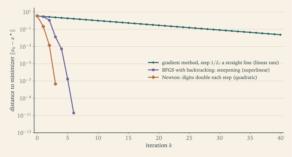
Figure 8.1 is the picture to remember when choosing among these methods. If iterations are cheap and moderate accuracy suffices, the straight line is acceptable. If high accuracy is needed or the problem is badly conditioned, the curved lines win by orders of magnitude, provided the cost per iteration in the table above can be afforded.
All three methods assume that the iterate may move freely. The next chapter puts back the constraints and the nondifferentiable terms, and shows how the gradient step can be adapted to both with one new operation.
Exercises
-
Compute the Newton step for \(f(x)=x_1^2+x_1x_2+x_2^2-3x_1\) at the point \((0,0)\) by solving the linear system of Definition 8.1 without forming an inverse, and verify that the step lands on the minimizer found in Example 3.4.
Answer
At \((0,0)\) the gradient is \((-3,0)\) and the Hessian is \(\begin{pmatrix}2&1\\1&2\end{pmatrix}\) . The system \(2d_1+d_2=3\) , \(d_1+2d_2=0\) gives \(d_2=-1\) , \(d_1=2\) , so \(x+d_{\mathrm N}=(2,-1)\) , the minimizer of Example 3.4. The function is quadratic, so one step suffices (Proposition 8.2(c)).
-
For \(f(x)=x-\log x\) on \(x>0\) derive the Newton iteration, show that the error \(e_k=1-x_k\) satisfies \(e_{k+1}=e_k^2\) exactly, compute four iterates from \(x_0=0.5\) , and determine the set of starting points from which the pure iteration converges.
Solution
Here \(f'(x)=1-1/x\) and \(f''(x)=1/x^2>0\) , so \(f\) is strictly convex on \(x>0\) with minimizer \(x^\star=1\) . The Newton step is \(-f'(x)/f''(x)=-(1-1/x)x^2=x-x^2\) , so
\[ x_{k+1}=x_k+x_k-x_k^2=2x_k-x_k^2 . \]For the error \(e_k=1-x_k\) : \(e_{k+1}=1-2x_k+x_k^2=(1-x_k)^2=e_k^2\) . The error is squared exactly at every step, with constant \(1\) .
From \(x_0=0.5\) , \(e_0=0.5\) , so the errors are \(0.25\) , \(0.0625\) , \(0.00390625\) , \(1.526\times10^{-5}\) and the iterates are
\[ x_1=0.75,\qquad x_2=0.9375,\qquad x_3=0.99609375,\qquad x_4\approx0.99998474 . \]Since \(e_k=e_0^{2^k}\) , the iteration converges if and only if \(\lvert e_0\rvert<1\) , that is, \(0<x_0<2\) . This also keeps the iterates in the domain: \(x_{k+1}=x_k(2-x_k)\) is positive exactly when \(0<x_k<2\) . At \(x_0=2\) the first step lands on \(0\) , outside the domain, and for \(x_0>2\) it lands on a negative number. So the basin of the pure method is the interval \((0,2)\) ; a line search that also rejects points outside the domain would extend convergence to every positive start.
-
Prove that the Newton decrement satisfies \(\tfrac12\lambda(x)^2=f(x)-\min_dq_x(d)\) , and evaluate \(\lambda(x)^2\) for \(f(x)=\tfrac12(x_1^2+4x_2^2)\) at \(x=(4,1)\) , comparing \(\tfrac12\lambda(x)^2\) with \(f(x)-f^\star\) .
Solution
Write \(g=\nabla f(x)\) and \(H=\nabla^2f(x)\succ 0\) . The model \(q_x(d)=f(x)+g^{\top}d+\tfrac12d^{\top}Hd\) is a strictly convex quadratic in \(d\) , minimized by Theorem 3.7(a) at \(d=-H^{-1}g\) . Its minimum value is
\[ f(x)-g^{\top}H^{-1}g+\tfrac12g^{\top}H^{-1}HH^{-1}g=f(x)-\tfrac12g^{\top}H^{-1}g=f(x)-\tfrac12\lambda(x)^2 . \]So \(f(x)-\min_dq_x(d)=\tfrac12\lambda(x)^2\) .
For \(f(x)=\tfrac12(x_1^2+4x_2^2)\) at \((4,1)\) : \(g=(4,4)\) and \(H\) is diagonal with entries \(1\) and \(4\) , so \(\lambda^2=16/1+16/4=20\) and \(\tfrac12\lambda^2=10\) . The true gap is \(f(4,1)-f^\star=8+2-0=10\) . They agree exactly because \(f\) is quadratic and the model is \(f\) itself. For a general function \(\tfrac12\lambda(x)^2\) is an estimate of \(f(x)-f^\star\) that becomes accurate near the minimizer, which is why \(\lambda(x)^2\le2\varepsilon\) is a natural stopping test for Newton’s method; unlike the gradient norm, it is unchanged by a linear change of variables.
-
Show that the pure Newton iteration for \(f(x)=x^6\) is \(x_{k+1}=\tfrac45x_k\) , state the kind of convergence this is, and identify the hypothesis of Theorem 8.3 that fails.
Answer
\(f'=6x^5\) and \(f''=30x^4\) , so \(x_{k+1}=x_k-x_k/5=\tfrac45x_k\) : linear convergence with factor \(0.8\) . The hypothesis \(m>0\) fails, since \(f''(0)=0\) .
-
For \(f(x)=\log(e^{x}+e^{-x})\) show that the pure Newton iteration is \(x_{k+1}=x_k-\tfrac12\sinh(2x_k)\) , and that it converges exactly when \(\lvert x_0\rvert<x_c\) , where \(x_c\approx1.0887\) is the positive solution of \(\sinh(2x)=4x\) .
Solution
With \(f(x)=\log(e^{x}+e^{-x})\) we get \(f'(x)=\tanh x\) and \(f''(x)=1/\cosh^2x\) . The Newton step is \(-\tanh x\cosh^2x=-\sinh x\cosh x=-\tfrac12\sinh(2x)\) , so \(x_{k+1}=\phi(x_k)\) with \(\phi(x)=x-\tfrac12\sinh(2x)\) .
The map \(\phi\) is odd, and for \(x>0\) it satisfies \(\phi(x)<x\) , because \(\sinh(2x)>0\) , and in fact \(\phi(x)<0\) , because \(\sinh(2x)>2x\) . So the iterates alternate in sign and \(\lvert x_{k+1}\rvert=\tfrac12\sinh(2\lvert x_k\rvert)-\lvert x_k\rvert\) . Hence \(\lvert x_{k+1}\rvert<\lvert x_k\rvert\) exactly when \(\sinh(2\lvert x_k\rvert)<4\lvert x_k\rvert\) . The function \(\sinh(2x)-4x\) is negative for small positive \(x\) (its derivative at \(0\) is \(-2\) ), is convex for \(x>0\) , and tends to infinity, so it has exactly one positive zero \(x_c\) ; numerically \(x_c\approx1.0887\) .
If \(\lvert x_0\rvert<x_c\) , the absolute values decrease and stay below \(x_c\) ; a decreasing sequence of nonnegative numbers has a limit \(a\) , which by continuity satisfies \(a=\tfrac12\sinh(2a)-a\) , and the only solution in \([0,x_c)\) is \(a=0\) . So the method converges. If \(\lvert x_0\rvert=x_c\) the iterates cycle between \(x_c\) and \(-x_c\) . If \(\lvert x_0\rvert>x_c\) the absolute values increase, and since there is no fixed value above \(x_c\) they diverge. The function is smooth and strictly convex, and still the pure method has a bounded basin.
-
For \(f(x)=e^{x}-2x\) at \(x_0=-3\) compute the Newton step, show that the full step increases \(f\) enormously, and carry out backtracking with \(c=0.25\) and \(\beta=0.5\) to find the accepted step size and the new point.
Solution
At \(x_0=-3\) : \(f'(x_0)=e^{-3}-2\approx-1.9502\) , \(f''(x_0)=e^{-3}\approx0.0498\) , and \(f(x_0)=e^{-3}+6\approx6.0498\) . The Newton step is \(d=-f'/f''\approx39.171\) . The curvature is tiny, so the model is very flat and its minimizer is far away.
The full step lands on \(x\approx36.17\) , where \(f\approx5\times10^{15}\) . The backtracking test is \(f(x_0+td)\le f(x_0)+0.25\,t\,f'(x_0)d\approx6.0498-19.098\,t\) .
\(t=1\) : \(f\approx5\times10^{15}\) , required \(\le-13.05\) . Fail. \(t=0.5\) : the point is \(16.59\) , \(f\approx1.6\times10^{7}\) , required \(\le-3.50\) . Fail. \(t=0.25\) : the point is \(6.79\) , \(f\approx877.8\) , required \(\le1.28\) . Fail. \(t=0.125\) : the point is \(1.896\) , \(f\approx2.869\) , required \(\le3.663\) . Pass.
The accepted step size is \(t=0.125\) and the new point is \(x_1\approx1.896\) . From there the pure iteration \(x-1+2e^{-x}\) gives \(1.197\) , \(0.801\) , \(0.699\) , and then converges quadratically to \(\log2\) as in Example 8.2. Three failed trials cost three function evaluations, far less than the damage the full step would have done.
-
For \(f(x)=x^3-3x\) at \(x=-0.5\) compute the Newton step and show that it moves toward the local maximizer \(x=-1\) ; explain this in terms of the sign of \(f''\) and the nature of the quadratic model.
Answer
\(f'(-0.5)=-2.25\) and \(f''(-0.5)=-3\) , so the step is \(-f'/f''=-0.75\) and the new point is \(-1.25\) , on the far side of the local maximizer \(-1\) , to which the iteration then converges. With \(f''<0\) the quadratic model is a downward parabola; its only stationary point is its maximum, and that is where the Newton step goes.
-
Explain why Newton’s method for minimizing \(f\) coincides with Newton’s root-finding method applied to \(\nabla f\) , and why this means the iteration can converge to a saddle point; illustrate by running three steps on \(f(x,y)=x^3-3x+y^2\) from \((-0.9,\,0.2)\) .
Hint
The Newton step solves the linearisation of \(\nabla f(x)=0\) , and the equation \(\nabla f=0\) does not know which kind of stationary point it describes. Here the variables decouple: \(x^+=(x^2+1)/(2x)\) and \(y^+=0\) . From \((-0.9,0.2)\) the iterates are \((-1.00556,0)\) , \((-1.0000154,0)\) , and then \((-1,0)\) to ten digits: the saddle of Example 3.1.
-
For \(f(x)=e^{x}-2x\) and the ball of radius \(r=0.2\) about \(x^\star=\log2\) , compute \(m\) and a valid Lipschitz constant \(M\) , check that \(m/(2M)\ge r\) , and verify the inequality of Theorem 8.3 for the Newton step taken from \(x=x^\star+0.2\) .
Solution
Here \(m=f''(x^\star)=e^{\log2}=2\) . On the ball \([x^\star-0.2,\ x^\star+0.2]\) , the Hessian \(f''(x)=e^{x}\) has derivative \(e^{x}\le e^{\log2+0.2}=2e^{0.2}\approx2.443\) , so by the mean value theorem \(\lvert f''(x)-f''(y)\rvert\le2.443\,\lvert x-y\rvert\) there. Take \(M=2.443\) . Then \(m/(2M)\approx0.409\ge0.2=r\) , so the theorem applies to every starting point in the ball.
Take \(x=x^\star+0.2\approx0.89315\) , with error \(e=0.2\) . Since \(e^{-x}=\tfrac12e^{-0.2}\approx0.40937\) , the Newton iterate is
\[ x^+=x-1+2e^{-x}\approx0.89315-1+0.81873=0.71188, \]with error \(\lvert x^+-x^\star\rvert\approx0.01873\) . The theorem’s bound is \(\tfrac Mm e^2=1.2214\cdot0.04\approx0.0489\) . Indeed \(0.01873\le0.0489\) , and also \(0.01873\le\tfrac12\cdot0.2\) . The observed ratio \(0.01873/0.04\approx0.47\) is close to the asymptotic constant \(\tfrac12\) of Example 8.2 and well inside the guaranteed constant, which had to allow for the worst behaviour of the Hessian anywhere in the ball.
-
Apply the secant method of Section 8.5 to \(f(x)=x-\log x\) starting from \(x_0=0.5\) and \(x_1=0.75\) , computing \(x_2\) and \(x_3\) , and compare the errors with those of the Newton iteration in Exercise 2.
Answer
With \(f'(x)=1-1/x\) : \(f'(0.5)=-1\) , \(f'(0.75)=-\tfrac13\) , \(b_1=(\tfrac23)/0.25=\tfrac83\) , so \(x_2=0.75+\tfrac13\cdot\tfrac38=0.875\) . Then \(f'(0.875)=-\tfrac17\) , \(b_2=(\tfrac13-\tfrac17)/0.125=\tfrac{32}{21}\) , and \(x_3=0.875+\tfrac17\cdot\tfrac{21}{32}=0.96875\) . The errors \(0.125\) and \(0.03125\) are each the product of the two preceding errors; Newton from \(0.75\) gives errors \(0.0625\) and \(0.0039\) .
-
For \(H=I\) , \(s=(1,0)\) , and \(y=(2,1)\) , compute the BFGS update \(H^+\) from Definition 8.6 and verify by direct calculation that it is symmetric, satisfies \(H^+y=s\) , and is positive definite.
Solution
Here \(y^{\top}s=2\cdot1+1\cdot0=2>0\) , so \(\rho=\tfrac12\) . Compute the two factors:
\[ I-\rho\,sy^{\top}=\begin{pmatrix}1&0\\0&1\end{pmatrix}-\tfrac12\begin{pmatrix}2&1\\0&0\end{pmatrix}=\begin{pmatrix}0&-\tfrac12\\0&1\end{pmatrix},\qquad I-\rho\,ys^{\top}=\begin{pmatrix}0&0\\-\tfrac12&1\end{pmatrix}. \]With \(H=I\) the first term of the update is their product, \(\begin{pmatrix}\tfrac14&-\tfrac12\\-\tfrac12&1\end{pmatrix}\) , and the second term is \(\rho\,ss^{\top}=\begin{pmatrix}\tfrac12&0\\0&0\end{pmatrix}\) . Therefore
\[ H^+=\begin{pmatrix}\tfrac34&-\tfrac12\\-\tfrac12&1\end{pmatrix}. \]It is symmetric. Secant equation: \(H^+y=(\tfrac34\cdot2-\tfrac12\cdot1,\ -\tfrac12\cdot2+1\cdot1)=(1,0)=s\) . Positive definiteness: the trace is \(\tfrac74>0\) and the determinant is \(\tfrac34-\tfrac14=\tfrac12>0\) , so both eigenvalues are positive. All three conclusions of Proposition 8.7 are confirmed. The update has reduced the first diagonal entry from \(1\) to \(\tfrac34\) : the gradient changed by \(2\) units along a step of \(1\) unit in the first coordinate, indicating curvature larger than \(1\) there, so the inverse-curvature estimate goes down.
-
Let \(f\) be differentiable and \(m\) -strongly convex. Prove that \((\nabla f(x)-\nabla f(z))^{\top}(x-z)\ge m\lVert x-z\rVert^2\) for all \(x,z\) , and deduce that the curvature condition \(y^{\top}s>0\) of Definition 8.6 holds for every nonzero step.
Solution
By Proposition 2.9, for all \(x,z\) ,
\[ f(z)\ge f(x)+\nabla f(x)^{\top}(z-x)+\frac m2\lVert z-x\rVert^2,\qquad f(x)\ge f(z)+\nabla f(z)^{\top}(x-z)+\frac m2\lVert x-z\rVert^2 . \]Add the two inequalities. The function values cancel, leaving
\[ 0\ge\nabla f(x)^{\top}(z-x)+\nabla f(z)^{\top}(x-z)+m\lVert x-z\rVert^2=-(\nabla f(x)-\nabla f(z))^{\top}(x-z)+m\lVert x-z\rVert^2, \]which is the claim. Now take \(x=x_{k+1}\) and \(z=x_k\) , so that \(x-z=s_k\) and \(\nabla f(x)-\nabla f(z)=y_k\) . The inequality reads \(y_k^{\top}s_k\ge m\lVert s_k\rVert^2\) , which is positive whenever \(s_k\ne 0\) . So on a strongly convex function every BFGS update is well defined and, by Proposition 8.7, preserves positive definiteness, whatever line search is used. The inequality proved here says that the gradient of a strongly convex function is strongly monotone; it is the multivariable version of the statement that \(f'\) increases at rate at least \(m\) .
-
A program computes each Newton step for a dense problem with \(n=5000\) variables as the product of an explicitly computed inverse Hessian with the gradient. Explain what is wasteful and what is risky about this, and say what should be computed instead.
Hint
Inverting costs about three times as much as a Cholesky factorization and yields a matrix that is then used only once, in a product with one vector; it also amplifies rounding errors more than triangular solves do. Factor the Hessian and solve two triangular systems. If the factorization breaks down, the Hessian was not positive definite, which is itself information the algorithm needs.
-
A dense strongly convex quadratic-like problem has \(n=1000\) variables. One gradient iteration costs about \(n^2\) operations and one Newton iteration about \(n^3/3\) . Estimate the total work for each method to reduce the error by a factor \(10^{-6}\) when \(\kappa=10^4\) and when \(\kappa=10\) , assuming Newton needs \(6\) iterations, and say which method is preferable in each case.
Solution
Use the estimate after Theorem 7.7: the squared error contracts by \(1-1/\kappa\) per gradient step, so reducing the error by \(10^{-6}\) , that is, the squared error by \(10^{-12}\) , takes about \(\kappa\log(10^{12})\approx27.6\,\kappa\) iterations.
For \(\kappa=10^4\) : about \(2.8\times10^{5}\) gradient iterations at \(n^2=10^6\) operations each, a total near \(2.8\times10^{11}\) . Newton: \(6\) iterations at \(n^3/3\approx3.3\times10^{8}\) each, a total near \(2\times10^{9}\) . Newton is cheaper by a factor of more than \(100\) .
For \(\kappa=10\) : about \(276\) gradient iterations, a total near \(2.8\times10^{8}\) , against the same \(2\times10^{9}\) for Newton. The gradient method is cheaper by a factor of about \(7\) .
The break-even is at \(\kappa\) near \(70\) for this problem size. The comparison omits the cost of forming the Hessian, which for a dense problem is of the same order as factoring it, and it assumes dense linear algebra; sparsity can make the Newton step far cheaper. The conclusion that survives such refinements is qualitative: the worse the conditioning and the higher the accuracy required, the stronger the case for second-order information, and quasi-Newton methods occupy the middle ground at \(n^2\) per iteration with no Hessian.
-
Theorem 8.3 assumes that \(\nabla^2f(x^\star)\) is positive definite. Use Theorem 3.4 to say what this implies about \(x^\star\) , and explain why observing that a Newton iteration has converged does not by itself show that the limit is a minimizer.
Hint
By Theorem 3.4 a stationary point with positive definite Hessian is a strict local minimizer, so the theorem’s hypotheses already guarantee what the limit is. Without that hypothesis the iteration is root finding on \(\nabla f\) , and Exercise 8.8 shows it converging to a saddle. Check the Hessian at the limit, or use a method that enforces decrease of \(f\) .
-
Let \(H\) be symmetric with smallest eigenvalue \(\mu\) , possibly negative, and let \(g\ne 0\) . Prove that for every \(\tau>-\mu\) the direction \(d=-(H+\tau I)^{-1}g\) satisfies \(g^{\top}d<0\) , and show that \(\tau d\to-g\) as \(\tau\to\infty\) .
Solution
Let \(\mu\) be the smallest eigenvalue of \(H\) and \(\tau>-\mu\) . The eigenvalues of \(H+\tau I\) are those of \(H\) shifted by \(\tau\) , so the smallest is \(\mu+\tau>0\) and \(H+\tau I\) is positive definite. The inverse of a positive definite matrix is positive definite, since its eigenvalues are the reciprocals. Therefore
\[ g^{\top}d=-g^{\top}(H+\tau I)^{-1}g<0\qquad\text{for }g\ne 0 . \]For the limit, factor out \(\tau\) : \(\tau d=-\tau(H+\tau I)^{-1}g=-\bigl(\tfrac1\tau H+I\bigr)^{-1}g\) . As \(\tau\to\infty\) the matrix \(\tfrac1\tau H+I\) tends to \(I\) , and matrix inversion is continuous at \(I\) , so \(\tau d\to-g\) . In words: for large \(\tau\) the modified direction is approximately \(-g/\tau\) , a short step along the negative gradient. For \(\tau\) just large enough to restore definiteness, it stays close to the Newton direction in the subspace where the curvature was already positive. The parameter \(\tau\) thus trades trust in the quadratic model against the safety of steepest descent, which is the idea behind trust-region methods.
-
Show that one pure Newton step for the least-squares objective \(\lVert Ax-b\rVert^2\) , with the columns of \(A\) independent, leads from any starting point to the solution of the normal equations, and relate this to Proposition 8.2(c).
Hint
The objective is the quadratic with \(P=2A^{\top}A\succ 0\) and \(q=-2A^{\top}b\) , so Proposition 8.2(c) applies: \(x+d_{\mathrm N}=-P^{-1}q=(A^{\top}A)^{-1}A^{\top}b\) .
-
Three algorithms report the error sequences (a) \(10^{-1},10^{-2},10^{-3},10^{-4}\) ; (b) \(10^{-1},10^{-2},10^{-4},10^{-8}\) ; (c) \(10^{-1},5\times10^{-2},3.3\times10^{-2},2.5\times10^{-2}\) . Classify each as sublinear, linear, or quadratic, and for each estimate the error after two more iterations.
Answer
(a) Linear with factor \(0.1\) ; next errors \(10^{-5}\) , \(10^{-6}\) . (b) Quadratic with \(e_{k+1}=e_k^2\) ; next errors \(10^{-16}\) , \(10^{-32}\) . (c) Sublinear, \(e_k\approx0.1/k\) ; next errors about \(2\times10^{-2}\) and \(1.7\times10^{-2}\) .
-
Apply the backtracking Newton iteration to \(f(x)=\tfrac12x^2\) from \(x_0=1\) with the inadmissible parameter \(c=0.75\) and with \(\beta=0.5\) : show that the step \(t=1\) is rejected and \(t=0.5\) accepted at every iteration, give the resulting rate of convergence, and explain why Definition 8.4 requires \(c<\tfrac12\) by finding the largest \(c\) for which the unit step is accepted on this function.
Solution
For \(f(x)=\tfrac12x^2\) the gradient is \(x\) and the Hessian is \(1\) , so the Newton step is \(d=-x\) and the decrement is \(\lambda(x)^2=x^2\) . A trial step \(t\) leads to \((1-t)x\) , and the sufficient-decrease test \(f(x+td)\le f(x)-c\,t\,\lambda(x)^2\) reads
\[ \tfrac12(1-t)^2x^2\le\tfrac12x^2-c\,t\,x^2 . \]For \(x\ne0\) , divide by \(x^2\) and expand: \(t^2-2t\le-2ct\) , that is, \(t\le2(1-c)\) . The test does not depend on \(x\) , so the same trials succeed and fail at every iteration.
With \(c=0.75\) the test is \(t\le0.5\) . The trial \(t=1\) fails; the next trial \(t=0.5\) passes, with equality. So every iteration takes \(t=0.5\) and \(x_{k+1}=\tfrac12x_k\) : from \(x_0=1\) the iterates are \(0.5\) , \(0.25\) , \(0.125\) , and the convergence is linear with factor \(\tfrac12\) , although the function is quadratic and a single full step would have reached the minimizer.
The unit step passes the test exactly when \(1\le2(1-c)\) , that is, when \(c\le\tfrac12\) . So \(\tfrac12\) is the largest admissible value on this function, and it is admissible here only because the quadratic model is exact, the full step decreasing \(f\) by exactly \(\tfrac12\lambda^2\) . For a general function the decrease achieved by a full step near the solution is \(\tfrac12\lambda^2\) up to a relative error that tends to zero but can have either sign, so the unit step is guaranteed to pass eventually only if \(c\) is strictly less than \(\tfrac12\) . That is the restriction in Definition 8.4, and it is a hypothesis of Theorem 8.5.