For a square matrix \(A\) the numbers \(\lambda\) at which \(A-\lambda I\) fails to be invertible are the eigenvalues, and for a symmetric matrix the eigenvectors can be chosen as an orthonormal basis in which \(A\) is diagonal. Everything one wants to know about \(A\) , its norm, its powers, the solvability of \(Ax-\lambda x=b\) , can be read from that diagonal form.

In infinite dimensions the first sentence breaks down. The right shift \(S\) on \(\ell^2\) has no eigenvalues whatever, and yet \(S-\lambda I\) fails to be invertible for every complex number \(\lambda\) in the closed unit disc. An operator can fail to be invertible by failing to be onto, or by having an inverse that is unbounded, without having any kernel. The set of all \(\lambda\) at which invertibility fails is the spectrum, and it is the correct generalisation of the set of eigenvalues. This chapter defines it, computes it for the standard examples, and then shows that for the operators closest to matrices the classical picture survives intact: a compact self-adjoint operator on a Hilbert space has an orthonormal basis of eigenvectors, with eigenvalues that are real and accumulate only at zero.

Throughout, scalars are complex, \(X\) is a nonzero complex Banach space, and \(H\) a complex Hilbert space. We write \(T-\lambda\) for \(T-\lambda I\) .

10.1 Resolvent set and spectrum

Every eigenvalue is an approximate eigenvalue, and every approximate eigenvalue belongs to the spectrum, since an invertible \(T-\lambda\) is bounded below. By Proposition 5.4 there are exactly three ways for \(\lambda\) to lie in \(\sigma(T)\) : \(T-\lambda\) has a kernel; or it is injective but not bounded below, so that \(\lambda\) is an approximate eigenvalue and the range is not closed; or it is bounded below but its range, though closed, is not all of \(X\) . In finite dimensions only the first can happen.

The number \(r(T)=\max\{\lvert\lambda\rvert:\lambda\in\sigma(T)\}\) is the spectral radius. The theorem shows \(r(T)\le\inf_n\lVert T^n\rVert^{1/n}\) ; in fact equality holds and the infimum is a limit, a formula of Gelfand that we shall not prove. The proof of nonemptiness used three earlier chapters at once: the Neumann series, the Hahn–Banach theorem in the form of Corollary 3.6, and, through continuity of the inverse, completeness.

10.2 Self-adjoint operators

For a self-adjoint operator the third way of belonging to the spectrum, bounded below with range not dense, never occurs. The multiplication operator of Example 10.2 is self-adjoint, and its spectrum \([0,1]\) is real and consists of approximate eigenvalues, as the proposition requires. Part (c) fails without self-adjointness (Exercise 8).

10.3 The spectrum of a compact operator

Statement (c) is the Fredholm alternative: for \(\lambda\ne 0\) , either the equation \(Tu-\lambda u=f\) has exactly one solution for every \(f\) , or the homogeneous equation \(Tu-\lambda u=0\) has a nonzero solution. Uniqueness implies existence, as for square matrices. When the second case holds, (b) and Proposition 8.4 say exactly which \(f\) are admissible: the equation is solvable if and only if \(f\) is orthogonal to \(\ker(T^*-\overline\lambda)\) . The restriction \(\lambda\ne 0\) is essential. The equation \(Tu=f\) with \(T\) compact is never solvable for all \(f\) (Exercise 4 of Chapter 9Chapter 9), and Example 10.3 shows that \(T\) can be injective all the same.

10.4 Diagonalising a compact self-adjoint operator

The supremum that defines the norm is attained, because compactness lets a maximizing sequence converge. This is the infinite-dimensional replacement for the argument that a continuous function on the compact unit sphere of \(\mathbb R^n\) has a maximum.

In the basis of eigenvectors \(T\) is the diagonal operator of Example 9.1. The theorem thus says that Example 9.1 is, up to a change of orthonormal basis, the only example of a compact self-adjoint operator. Three consequences are immediate. The norm is the largest \(\lvert\lambda_k\rvert\) . The best approximation of \(T\) by an operator of rank \(n\) obtained from the expansion has error \(\lvert\lambda_{n+1}\rvert\) . And equations can be solved coordinate by coordinate: for \(\mu\ne 0\) different from every \(\lambda_k\) , and \(f=f_0+\sum_k\langle f,e_k\rangle e_k\) with \(f_0\in\ker T\) , the unique solution of \(Tu-\mu u=f\) is

When \(\mu\) equals some \(\lambda_j\) the formula shows the Fredholm alternative explicitly: the coefficient \(\langle f,e_k\rangle/(\lambda_k-\mu)\) is undefined for the indices with \(\lambda_k=\mu\) unless \(\langle f,e_k\rangle=0\) for those indices, in which case that coefficient of \(u\) is arbitrary.

The theorem also reaches operators that are not self-adjoint. If \(T\) is any compact operator on \(H\) , then \(T^*T\) is compact, self-adjoint, and has nonnegative eigenvalues, since \(\langle T^*Tx,x\rangle=\lVert Tx\rVert^2\) . Their square roots \(s_1\ge s_2\ge\cdots\) are the singular values of \(T\) , and by Theorem 8.3

This is the promised extension of the formula for the Euclidean norm of a matrix in Section 2.2.

Example 10.5: The eigenvalues of an integral operator

Let \((Kf)(x)=\int_0^1\min\{x,y\}f(y)\,dy\) on \(L^2[0,1]\) . The kernel is real and symmetric, so \(K\) is self-adjoint, and it is compact by Example 9.2. To find its eigenvalues write

\[ (Kf)(x)=\int_0^xyf(y)\,dy+x\int_x^1f(y)\,dy,\qquad(Kf)'(x)=\int_x^1f(y)\,dy,\qquad(Kf)''(x)=-f(x). \]

First, \(Kf=0\) implies \(f=-(Kf)''=0\) , so \(\ker K=\{0\}\) . If \(Ku=\lambda u\) with \(\lambda\ne 0\) , then \(u=\lambda^{-1}Ku\) is twice differentiable and

\[ \lambda u''=-u,\qquad u(0)=0,\qquad u'(1)=0 , \]

the boundary conditions being read off from the formulas for \(Ku\) and \((Ku)'\) . For \(\lambda<0\) the solutions with \(u(0)=0\) are multiples of a hyperbolic sine, whose derivative never vanishes. For \(\lambda>0\) they are multiples of \(\sin(x/\sqrt\lambda)\) , and \(u'(1)=0\) requires \(\cos(1/\sqrt\lambda)=0\) . Hence

\[ \lambda_k=\frac{1}{(k-\tfrac12)^2\pi^2}=\frac{4}{(2k-1)^2\pi^2},\qquad e_k(x)=\sqrt2\,\sin\bigl((k-\tfrac12)\pi x\bigr),\qquad k=1,2,3,\dots \]

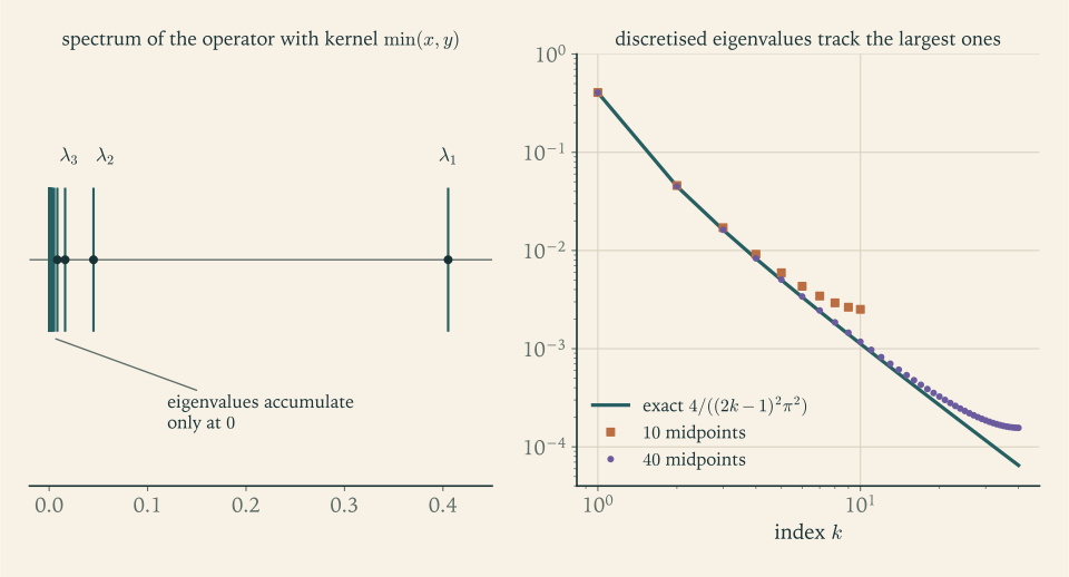
The first four eigenvalues are approximately \(0.4053\) , \(0.0450\) , \(0.0162\) , and \(0.0083\) . They decrease like \(k^{-2}\) and accumulate at \(0\) , which belongs to the spectrum without being an eigenvalue.

By Theorem 10.6 with \(\ker K=\{0\}\) , the functions \(e_k\) form an orthonormal basis of \(L^2[0,1]\) : completeness of this family of sines is a consequence of the spectral theorem and need not be proved separately. The norm is \(\lVert K\rVert=\lambda_1=4/\pi^2\approx 0.4053\) , as announced in Example 9.2. And since \(K\) is diagonal with entries \(\lambda_k\) in this basis, expanding the kernel gives \(\sum_k\lambda_k^2=\lVert k\rVert_{L^2}^2\) ; indeed

\[ \sum_{k\ge 1}\frac{16}{(2k-1)^4\pi^4}=\frac{16}{\pi^4}\cdot\frac{\pi^4}{96}=\frac16 , \]

the value computed directly in Example 9.2.

A computer finds these eigenvalues by replacing the integral with a sum over \(n\) midpoints, which turns \(K\) into an \(n\times n\) symmetric matrix. With \(n=10\) the three largest eigenvalues of the matrix are \(0.4061\) , \(0.0459\) , and \(0.0171\) ; with \(n=40\) they are \(0.40534\) , \(0.04508\) , and \(0.01626\) . Because \(K\) is compact, it is a norm limit of finite-rank operators, and the eigenvalues of the discretisations converge to those of \(K\) . Contrast Example 10.1, where the truncations of a non-compact operator carried no information about its spectrum.

Exercises

1. Let \((Dx)_k=d_kx_k\) on \(\ell^2\) with \((d_k)\) bounded. Prove that the eigenvalues of \(D\) are the numbers \(d_k\) and that \(\sigma(D)\) is the closure of \(\{d_k\}\) ; describe the spectrum for \(d_k=1/k\) .

   Solution

   Eigenvalues. \(De_k=d_ke_k\) , so each \(d_k\) is an eigenvalue. Conversely if \(Dx=\lambda x\) with \(x\ne 0\) , then \((d_k-\lambda)x_k=0\) for all \(k\) , and choosing \(k\) with \(x_k\ne 0\) gives \(\lambda=d_k\) .

   Spectrum. Let \(\Lambda\) be the closure of \(\{d_k\}\) . If \(\lambda\notin\Lambda\) , then \(\delta=\inf_k\lvert d_k-\lambda\rvert>0\) , and the diagonal operator with entries \((d_k-\lambda)^{-1}\) is bounded, with norm \(1/\delta\) by Exercise 3 of Chapter 2Chapter 2; it is a two-sided inverse of \(D-\lambda\) . So \(\lambda\in\rho(D)\) , and \(\sigma(D)\subseteq\Lambda\) . If \(\lambda\in\Lambda\) , either \(\lambda=d_k\) for some \(k\) , an eigenvalue, or there are indices \(k_j\) with \(d_{k_j}\to\lambda\) , and then

   \[ \lVert(D-\lambda)e_{k_j}\rVert=\lvert d_{k_j}-\lambda\rvert\to 0 , \]

   so \(\lambda\) is an approximate eigenvalue. Either way \(\lambda\in\sigma(D)\) . Hence \(\sigma(D)=\Lambda\) .

   The case \(d_k=1/k\) . The spectrum is \(\{0\}\cup\{1/k:k\ge 1\}\) . Each \(1/k\) is an eigenvalue with eigenvector \(e_k\) . The point \(0\) is in the spectrum as the limit of the eigenvalues, an approximate eigenvalue with approximate eigenvectors \(e_k\) , but it is not an eigenvalue, since \(D\) is injective. This is the model for Theorem 10.4: a compact operator whose nonzero spectrum is a sequence of eigenvalues converging to \(0\) .

2. Let \(P\) be an orthogonal projection on \(H\) with \(P\ne 0\) and \(P\ne I\) . Find \(\sigma(P)\) and verify the formula \((P-\lambda)^{-1}=-\tfrac1\lambda(I-P)+\tfrac1{1-\lambda}P\) for \(\lambda\notin\{0,1\}\) .

   Answer

   \(\sigma(P)=\{0,1\}\) , both eigenvalues, with eigenspaces \(\ker P\) and \(\operatorname{ran}P\) . For the formula use \(P(I-P)=0\) and \(P^2=P\) : \((P-\lambda)(I-P)=-\lambda(I-P)\) and \((P-\lambda)P=(1-\lambda)P\) , so the product of \(P-\lambda\) with the proposed inverse is \((I-P)+P=I\) .

3. Prove that \(\sigma(T^*)=\{\overline\lambda:\lambda\in\sigma(T)\}\) for \(T\in\mathcal B(H)\) .

   Hint

   \((T-\lambda)^*=T^*-\overline\lambda\) , and an operator \(A\) is invertible if and only if \(A^*\) is, with \((A^*)^{-1}=(A^{-1})^*\) .

4. For the left shift \(L\) on \(\ell^2\) and \(\lvert\lambda\rvert=1\) , show that \(\lambda\) is not an eigenvalue but is an approximate eigenvalue, using the unit vectors \(u_n=n^{-1/2}(1,\lambda,\dots,\lambda^{n-1},0,\dots)\) .

   Solution

   Not an eigenvalue. If \(Lx=\lambda x\) then \(x_{k+1}=\lambda x_k\) for all \(k\) , so \(x=x_1(1,\lambda,\lambda^2,\dots)\) . When \(\lvert\lambda\rvert=1\) every coordinate has modulus \(\lvert x_1\rvert\) , and such a sequence is in \(\ell^2\) only if \(x_1=0\) . So \(\ker(L-\lambda)=\{0\}\) .

   Approximate eigenvalue. The vector \(u_n\) has \(n\) nonzero coordinates, each of modulus \(n^{-1/2}\) , so \(\lVert u_n\rVert=1\) . We compute

   \[ Lu_n=n^{-1/2}(\lambda,\lambda^2,\dots,\lambda^{n-1},0,\dots),\qquad\lambda u_n=n^{-1/2}(\lambda,\lambda^2,\dots,\lambda^{n-1},\lambda^n,0,\dots). \]

   They agree in the first \(n-1\) coordinates, and

   \[ (L-\lambda)u_n=-n^{-1/2}\lambda^n e_n,\qquad\lVert(L-\lambda)u_n\rVert=n^{-1/2}\to 0 . \]

   So \(\lambda\) is an approximate eigenvalue, and \(\lambda\in\sigma(L)\) . For \(n=100\) the residual is \(0.1\) . The vectors \(u_n\) are normalised truncations of the would-be eigenvector \((1,\lambda,\lambda^2,\dots)\) , which just fails to be square-summable. Inside the open disc the same sequence is a genuine eigenvector; on the boundary circle only approximate eigenvectors remain, and the convergence \(n^{-1/2}\) is slow, reflecting that the points of the circle lie on the edge of the spectrum.

5. Compute \(\lVert A^n\rVert^{1/n}\) for \(n=1,2,4,8\) in the Euclidean norm, to three decimals, for \(A=\begin{pmatrix}1&1\\0&1\end{pmatrix}\) , given that \(A^n=\begin{pmatrix}1&n\\0&1\end{pmatrix}\) , and compare the limit with the spectral radius and with \(\lVert A\rVert\) .

   Answer

   The largest singular value of \(\begin{pmatrix}1&n\\0&1\end{pmatrix}\) is \(\tfrac12(n+\sqrt{n^2+4})\) . So \(\lVert A^n\rVert^{1/n}\) is \(1.618\) , \(1.554\) , \(1.435\) , \(1.299\) for \(n=1,2,4,8\) , decreasing toward \(1\) . The spectral radius is \(1\) , the only eigenvalue, while \(\lVert A\rVert=1.618\) ; the norms of the powers grow like \(n\) , which is slower than any exponential.

6. Let \(\varphi\in C[0,1]\) be real-valued and \(M_\varphi f=\varphi f\) on \(L^2[0,1]\) . Show that \(\sigma(M_\varphi)=\varphi([0,1])\) , and give a condition on \(\varphi\) under which \(M_\varphi\) has an eigenvalue.

   Hint

   If \(\lambda\notin\varphi([0,1])\) , then \(1/(\varphi-\lambda)\) is bounded and multiplication by it inverts \(M_\varphi-\lambda\) . If \(\lambda=\varphi(x_0)\) , use normalised indicator functions of small intervals around \(x_0\) and continuity of \(\varphi\) . An eigenvalue \(\lambda\) exists exactly when the level set \(\{\varphi=\lambda\}\) has positive measure, for instance when \(\varphi\) is constant on an interval.

7. Prove directly that a self-adjoint operator has only real eigenvalues and that eigenvectors for distinct eigenvalues are orthogonal, and give a \(2\times 2\) matrix that is not self-adjoint and has two non-orthogonal eigenvectors.

   Answer

   See the proof of Proposition 10.3(a). The matrix \(\begin{pmatrix}1&1\\0&2\end{pmatrix}\) has eigenvalues \(1\) and \(2\) with eigenvectors \((1,0)\) and \((1,1)\) , whose inner product is \(1\) .

8. For \(A=\begin{pmatrix}0&1\\0&0\end{pmatrix}\) on \(\mathbb C^2\) compute \(\lVert A\rVert\) and \(\sup\{\lvert\langle Ax,x\rangle\rvert:\lVert x\rVert=1\}\) , and conclude that Proposition 10.3(c) requires self-adjointness.

   Solution

   Since \(Ax=(x_2,0)\) , \(\lVert Ax\rVert=\lvert x_2\rvert\le\lVert x\rVert\) with equality at \(x=e_2\) . So \(\lVert A\rVert=1\) .

   For the quadratic form, \(\langle Ax,x\rangle=x_2\overline{x_1}\) , and by the inequality between geometric and arithmetic means

   \[ \lvert\langle Ax,x\rangle\rvert=\lvert x_1\rvert\lvert x_2\rvert\le\tfrac12\bigl(\lvert x_1\rvert^2+\lvert x_2\rvert^2\bigr)=\tfrac12\lVert x\rVert^2 , \]

   with equality when \(\lvert x_1\rvert=\lvert x_2\rvert\) , for example at \(x=(1,1)/\sqrt2\) . Hence

   \[ \sup\{\lvert\langle Ax,x\rangle\rvert:\lVert x\rVert=1\}=\tfrac12<1=\lVert A\rVert . \]

   The identity \(\lVert T\rVert=\sup\lvert\langle Tx,x\rangle\rvert\) of Proposition 10.3(c) fails for this \(A\) , which is not self-adjoint: \(A^*=\begin{pmatrix}0&0\\1&0\end{pmatrix}\ne A\) . In the proof of (c), self-adjointness was used to turn \(\langle Tx,y\rangle+\langle Ty,x\rangle\) into \(2\operatorname{Re}\langle Tx,y\rangle\) . Note also that the spectrum of \(A\) is \(\{0\}\) , so neither the spectral radius, which is \(0\) , nor the quadratic form, which gives \(\tfrac12\) , recovers the norm \(1\) ; the singular values of \(A\) , which are \(1\) and \(0\) , do.

9. Find all eigenvalues and eigenfunctions of the operator on \(L^2[0,1]\) with kernel \(1-\max\{x,y\}\) , by reducing the eigenvalue equation to a boundary value problem as in Example 10.5.

   Solution

   Let \(W\) be the operator with kernel \(1-\max\{x,y\}\) . Splitting the integral at \(y=x\) ,

   \[ (Wf)(x)=(1-x)\int_0^xf(y)\,dy+\int_x^1(1-y)f(y)\,dy . \]

   Differentiating, the two boundary terms \(\pm(1-x)f(x)\) cancel, and

   \[ (Wf)'(x)=-\int_0^xf(y)\,dy,\qquad(Wf)''(x)=-f(x),\qquad(Wf)(1)=0,\qquad(Wf)'(0)=0 . \]

   In particular \(Wf=0\) forces \(f=0\) , so \(0\) is not an eigenvalue. If \(Wu=\lambda u\) with \(\lambda\ne 0\) , then \(u=\lambda^{-1}Wu\) is twice differentiable and satisfies

   \[ \lambda u''=-u,\qquad u'(0)=0,\qquad u(1)=0 . \]

   For \(\lambda<0\) the solutions with \(u'(0)=0\) are multiples of a hyperbolic cosine, which has no zero. For \(\lambda>0\) they are multiples of \(\cos(x/\sqrt\lambda)\) , and \(u(1)=0\) requires \(\cos(1/\sqrt\lambda)=0\) , that is, \(1/\sqrt\lambda=(k-\tfrac12)\pi\) . Therefore

   \[ \lambda_k=\frac{4}{(2k-1)^2\pi^2},\qquad e_k(x)=\sqrt2\cos\bigl((k-\tfrac12)\pi x\bigr),\qquad k\ge 1 . \]

   Conversely each such function satisfies the boundary value problem, and integrating \(-\lambda_ke_k''=e_k\) twice with the two boundary conditions recovers \(We_k=\lambda_ke_k\) . The eigenvalues coincide with those of the kernel \(\min\{x,y\}\) in Example 10.5, and the eigenfunctions are obtained from those by the reflection \(x\mapsto 1-x\) up to sign. This is as it must be: by Exercise 6 of Chapter 8Chapter 8 the two operators are \(V^*V\) and \(VV^*\) , which always have the same nonzero eigenvalues.

10. Let \(G\) be the operator on \(L^2[0,1]\) with kernel \(g(x,y)=\min\{x,y\}-xy\) . Show that \(u=Gf\) solves \(-u''=f\) , \(u(0)=u(1)=0\) , find the eigenvalues and eigenfunctions of \(G\) , and verify that \(\sum_k\lambda_k=\int_0^1g(x,x)\,dx\) .

    Solution

    Splitting at \(y=x\) , where \(\min\{x,y\}-xy\) equals \(y(1-x)\) for \(y\le x\) and \(x(1-y)\) for \(y\ge x\) ,

    \[ u(x)=(Gf)(x)=(1-x)\int_0^xyf(y)\,dy+x\int_x^1(1-y)f(y)\,dy . \]

    Clearly \(u(0)=0\) and \(u(1)=0\) . Differentiating, the terms \(\pm x(1-x)f(x)\) cancel:

    \[ u'(x)=-\int_0^xyf(y)\,dy+\int_x^1(1-y)f(y)\,dy,\qquad u''(x)=-xf(x)-(1-x)f(x)=-f(x). \]

    So \(u=Gf\) solves \(-u''=f\) with \(u(0)=u(1)=0\) ; \(G\) is the solution operator of this boundary value problem, and its kernel is the Green’s function.

    If \(Gu=\lambda u\) with \(\lambda\ne 0\) then \(\lambda u''=-u\) and \(u(0)=u(1)=0\) . Negative \(\lambda\) gives hyperbolic sines, which vanish only at \(0\) . Positive \(\lambda\) gives \(\sin(x/\sqrt\lambda)\) with \(\sin(1/\sqrt\lambda)=0\) :

    \[ \lambda_k=\frac1{k^2\pi^2},\qquad e_k(x)=\sqrt2\sin(k\pi x),\qquad k\ge 1 . \]

    Also \(Gf=0\) implies \(f=-(Gf)''=0\) , so \(0\) is not an eigenvalue and, by Theorem 10.6, the functions \(\sqrt2\sin(k\pi x)\) form an orthonormal basis of \(L^2[0,1]\) . This proves the completeness that Example 7.6 took for granted.

    Finally

    \[ \sum_{k\ge 1}\lambda_k=\frac1{\pi^2}\sum_{k\ge 1}\frac1{k^2}=\frac1{\pi^2}\cdot\frac{\pi^2}{6}=\frac16,\qquad\int_0^1g(x,x)\,dx=\int_0^1(x-x^2)\,dx=\frac12-\frac13=\frac16 . \]

    The sum of the eigenvalues equals the integral of the kernel along the diagonal, the analogue of the trace of a matrix.

11. For the operator on \(L^2[0,1]\) with kernel \(x+y\) , whose nonzero eigenvalues are \(\tfrac12\pm\tfrac1{\sqrt3}\) , determine all real \(\mu\) for which \(u-\mu Ku=f\) has exactly one solution for every \(f\in L^2[0,1]\) .

    Answer

    \(u-\mu Ku=f\) is uniquely solvable for every \(f\) exactly when \(1/\mu\) is not a nonzero eigenvalue of \(K\) . The exceptional values are \(\mu=(\tfrac12+\tfrac1{\sqrt3})^{-1}=4\sqrt3-6\approx 0.928\) and \(\mu=(\tfrac12-\tfrac1{\sqrt3})^{-1}=-(4\sqrt3+6)\approx-12.93\) . For every other real \(\mu\) there is exactly one solution.

12. Find the flaw: “Every \(n\times n\) truncation of the right shift is nilpotent, with spectrum \(\{0\}\) . Letting \(n\to\infty\) , the spectrum of \(S\) is \(\{0\}\) .”

    Answer

    The spectrum of a limit is not the limit of the spectra unless the convergence is in operator norm and further hypotheses hold. The truncations \(P_nSP_n\) converge to \(S\) only strongly; \(\lVert S-P_nSP_n\rVert=1\) for all \(n\) . In fact \(\sigma(S)\) is the closed unit disc (Example 10.1). For compact operators the truncations converge in norm, and then the argument is sound away from \(0\) .

13. Give examples of compact operators on \(\ell^2\) for which \(0\) is, respectively, an eigenvalue of infinite multiplicity, an eigenvalue of multiplicity one, and not an eigenvalue, and explain why \(0\) is in the spectrum in all three cases.

    Answer

    Infinite multiplicity: \(Tx=x_1e_1\) , whose kernel is the closed span of \(e_2,e_3,\dots\) . Multiplicity one: the diagonal operator with entries \(0,\tfrac12,\tfrac13,\tfrac14,\dots\) . Not an eigenvalue: the diagonal operator with entries \(1/k\) . In every case \(0\in\sigma(T)\) because a compact operator on an infinite-dimensional space cannot have a bounded inverse.

14. Let \(T\) be a compact self-adjoint operator with \(\langle Tx,x\rangle\ge 0\) for all \(x\) and eigenvalues \(\lambda_1\ge\lambda_2\ge\cdots>0\) as in Theorem 10.6. Prove that \(\lambda_1=\max\{\langle Tx,x\rangle:\lVert x\rVert=1\}\) and \(\lambda_2=\max\{\langle Tx,x\rangle:\lVert x\rVert=1,\ x\perp e_1\}\) .

    Hint

    Expand \(x=x_0+\sum_k\langle x,e_k\rangle e_k\) with \(x_0\in\ker T\) ; then \(\langle Tx,x\rangle=\sum_k\lambda_k\lvert\langle x,e_k\rangle\rvert^2\le\lambda_1\lVert x\rVert^2\) , with equality at \(e_1\) . For the second statement drop the term \(k=1\) .

15. With \(T\) as in Exercise 14, define \(Rx=\sum_k\sqrt{\lambda_k}\langle x,e_k\rangle e_k\) . Prove that \(R\) is compact and self-adjoint with \(R^2=T\) .

    Hint

    \(R\) is a norm limit of finite-rank operators since \(\sqrt{\lambda_k}\to 0\) , as in Theorem 10.6; it is self-adjoint because the coefficients are real; and \(R^2e_k=\lambda_ke_k\) while \(R\) and \(T\) both vanish on \(\ker T\) .

16. Let \(K\) be a compact self-adjoint integral operator on \(L^2[0,1]\) with kernel \(k\in L^2([0,1]^2)\) and eigen-expansion as in Theorem 10.6. Show that \(\sum_k\lambda_k^2=\lVert k\rVert_{L^2}^2\) , by expanding \(k\) in the orthonormal family \(e_i(x)\overline{e_j(y)}\) .

    Hint

    Complete \((e_k)\) to an orthonormal basis of \(L^2[0,1]\) by a basis of \(\ker K\) . The coefficient of \(k\) along \(e_i(x)\overline{e_j(y)}\) is \(\langle Ke_j,e_i\rangle\) , which is \(\lambda_i\) if \(i=j\) indexes an eigenvector with nonzero eigenvalue and \(0\) otherwise. Apply Parseval’s identity in \(L^2\) of the square.

17. Solve \(u(x)-\int_0^1\min\{x,y\}u(y)\,dy=x\) by converting it to a boundary value problem, verify the solution, and determine all \(\mu>0\) for which \(u-\mu Ku=f\) fails to be uniquely solvable.

    Solution

    Write the equation as \(u=x+Ku\) . By the formulas of Example 10.5, \((Ku)(0)=0\) , \((Ku)'(1)=0\) , and \((Ku)''=-u\) . Hence a solution is twice differentiable and satisfies

    \[ u''=-u,\qquad u(0)=0,\qquad u'(1)=1 . \]

    The first two conditions give \(u=c\sin x\) , and the third gives \(c\cos 1=1\) . So

    \[ u(x)=\frac{\sin x}{\cos 1}\approx 1.8508\,\sin x . \]

    Verification. \(\int_0^xy\sin y\,dy=\sin x-x\cos x\) and \(x\int_x^1\sin y\,dy=x\cos x-x\cos 1\) , so \(K(\sin)(x)=\sin x-x\cos 1\) . Then \(u-Ku=\frac{1}{\cos 1}\bigl(\sin x-\sin x+x\cos 1\bigr)=x\) , as required.

    Unique solvability. The equation \(u-\mu Ku=f\) is \((K-\tfrac1\mu)u=-\tfrac1\mu f\) . By Theorem 10.4 it is uniquely solvable for every \(f\) exactly when \(\tfrac1\mu\) is not an eigenvalue of \(K\) . The eigenvalues are \(\lambda_k=4/((2k-1)^2\pi^2)\) , so the exceptional values are

    \[ \mu_k=\frac{(2k-1)^2\pi^2}{4}:\qquad\mu_1\approx 2.467,\quad\mu_2\approx 22.2,\quad\mu_3\approx 61.7,\ \dots \]

    The value \(\mu=1\) used above is not among them. In the differential formulation these are the values for which \(u''+\mu u=0\) , \(u(0)=0\) , \(u'(1)=0\) has a nonzero solution, the resonant frequencies of the boundary value problem.

18. Use the Neumann series of Chapter 2 to show directly that the Volterra operator on \(L^2[0,1]\) has no nonzero eigenvalue, and deduce from Lemma 10.5 that \(V\) is not self-adjoint without computing \(V^*\) .

    Solution

    Let \(\lambda\ne 0\) . Then \(V-\lambda=-\lambda(I-\lambda^{-1}V)\) . By Example 10.3, \(\lVert V^n\rVert\le 1/(n-1)!\) on \(L^2[0,1]\) for \(n\ge 1\) , so

    \[ \sum_{n\ge 0}\lVert(\lambda^{-1}V)^n\rVert\le 1+\sum_{n\ge 1}\frac{\lvert\lambda\rvert^{-n}}{(n-1)!}<\infty . \]

    By Theorem 2.7, \(I-\lambda^{-1}V\) is invertible, hence so is \(V-\lambda\) . In particular \(V-\lambda\) is injective, and \(\lambda\) is not an eigenvalue. Together with the injectivity of \(V\) itself, this shows that \(V\) has no eigenvalues at all.

    Now suppose \(V\) were self-adjoint. It is compact and nonzero, since \(V1=x\ne 0\) . Lemma 10.5 would then make \(\lVert V\rVert\) or \(-\lVert V\rVert\) an eigenvalue, and \(\lVert V\rVert\ne 0\) . That contradicts the first part. Hence \(V\ne V^*\) . No formula for \(V^*\) was used: the absence of eigenvalues is by itself incompatible with being a nonzero compact self-adjoint operator. The same reasoning shows that any nonzero compact operator with spectrum \(\{0\}\) fails to be self-adjoint, and more generally fails to be normal.