A regional retailer must decide how many units of a seasonal product to order before the season starts. Demand will be high or low, and the retailer thinks the two are equally likely. Two firms offer demand forecasts at the same price. Forecast A is right four times out of five in either kind of season. Forecast B never misses a high season, but in a low season it still predicts high demand half of the time. Forecast A is right more often on average, so it looks like the better product. Yet the retailer orders for several product lines, each with its own margin, and next year it may face a different ordering problem altogether. The question it would like answered is not “which forecast is more accurate” but “is one forecast better for every decision we might face?”

That question has a precise answer, and the answer for these two forecasts is no: there are decisions for which A is worth twice as much as B, and others for which A is worth nothing and B is worth something. The tools of this chapter explain why. Chapter 1 summarized an experiment by its distribution of posteriors (Definition 1.2) and showed that the only restriction on that distribution is Bayes plausibility (Proposition 1.3): the posteriors average to the prior. It also claimed, without proof, that two experiments with the same distribution of posteriors are equally useful to every decision maker. Here we prove that claim, measure how useful an experiment is, and characterize when one experiment is more useful than another for all decision makers at once. The characterization is Blackwell’s theorem. Its hard direction is a duality argument, and the dual variables of that argument turn out to be a decision problem: whenever one experiment fails to dominate another, a linear program hands us a concrete decision maker who prefers the second.

Two ideas carry the chapter. The first is that a decision maker’s best attainable payoff is a convex function of her belief, and convexity is exactly what makes information valuable. The second is that “more informative” has a mechanical meaning: one experiment is more informative than another when the second can be manufactured from the first by adding noise. The theorem says that these two ideas, together with a geometric spreading condition on posteriors, all describe the same order.

2.1 Beliefs priced by the best action

A decision maker who must act under uncertainty cares about her belief only through what she can achieve with it. We start by making that dependence explicit.

The value \(U\) depends on the decision problem but not on any prior; it answers the question “if I held belief \(\mu\) and had to act now, how well would I do?” For each fixed action the map \(\mu\mapsto E_\mu[u(a,\omega)]\) is linear in the coordinates \(\mu(\omega)\) , because it is a weighted sum of the fixed numbers \(u(a,\omega)\) . The value of a belief is the upper envelope of these linear functions, one per action, and everything else in this section follows from that picture.

The convexity in (a) has a direct reading. A belief that is a mixture of \(\mu\) and \(\nu\) forces one action to serve both components, while a decision maker who knew which component she was in could tailor her action to each. Tailoring cannot hurt. That one-line intuition is the entire source of the value of information, and Proposition 2.3 below makes it exact.

The regions in (c) partition the simplex up to their boundaries. Ties sit on the boundaries: a belief on the common face of \(R(a)\) and \(R(b)\) makes the decision maker indifferent. If two actions have payoff vectors that differ by a nonzero constant, one of them is never optimal; if they have identical payoff vectors, their regions coincide, and we may delete one copy without changing \(U\) .

Example 2.1: Stock or skip

A shop decides whether to stock a new item (\(a=1\) ) or skip it (\(a=0\) ). The state is binary, \(\Omega=\{0,1\}\) , with \(\omega=1\) meaning the item sells well, and we identify a belief with the number \(\mu=\Pr(\omega=1)\) . Stocking earns \(3\) if the item sells and loses \(2\) if it does not; skipping earns \(0\) . Thus

\[ \ell_1(\mu)=3\mu-2(1-\mu)=5\mu-2,\qquad \ell_0(\mu)=0,\qquad U(\mu)=\max\{0,\,5\mu-2\}. \]

The shop stocks exactly when \(\mu\ge\tfrac25\) , and the regions are \(R(0)=[0,\tfrac25]\) and \(R(1)=[\tfrac25,1]\) , meeting at the indifference belief \(\tfrac25\) . The graph of \(U\) is flat at height \(0\) and then rises with slope \(5\) : a convex function with one kink.

Let the prior be \(\mu_0=\tfrac13\) . Then \(U(\mu_0)=\max\{0,-\tfrac13\}=0\) : without information the shop skips. Now a test market reports \(h\) (high) with probability \(\tfrac34\) when \(\omega=1\) and with probability \(\tfrac14\) when \(\omega=0\) , and reports \(l\) otherwise. By the posterior formula of Chapter 1,

\[ \pi(h)=\tfrac13\cdot\tfrac34+\tfrac23\cdot\tfrac14=\tfrac{5}{12},\qquad \mu_h=\frac{\tfrac13\cdot\tfrac34}{\tfrac{5}{12}}=\tfrac35,\qquad \pi(l)=\tfrac{7}{12},\qquad \mu_l=\frac{\tfrac13\cdot\tfrac14}{\tfrac{7}{12}}=\tfrac17 . \]

Bayes plausibility holds: \(\tfrac{5}{12}\cdot\tfrac35+\tfrac{7}{12}\cdot\tfrac17=\tfrac14+\tfrac{1}{12}=\tfrac13\) . After \(h\) the shop stocks and expects \(U(\tfrac35)=1\) ; after \(l\) it skips and expects \(0\) . Its expected payoff with the test is \(\tfrac{5}{12}\cdot 1+\tfrac{7}{12}\cdot 0=\tfrac{5}{12}\) , against \(0\) without it, so the test is worth \(\tfrac{5}{12}\) . As a cross-check, compute directly with the rule “stock after \(h\) ”: it earns \(3\) on the event \(\{\omega=1,h\}\) , of probability \(\tfrac14\) , and loses \(2\) on \(\{\omega=0,h\}\) , of probability \(\tfrac16\) , for \(\tfrac34-\tfrac13=\tfrac{5}{12}\) .

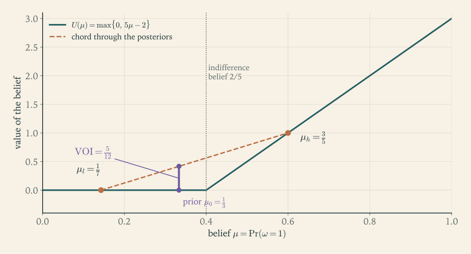
Figure 2.1 shows the computation as geometry. The expected payoff with the test is a weighted average of \(U\) at the two posteriors, with weights that make the posteriors average to the prior; that average is the height of the chord above \(\mu_0\) . The value without the test is the height of the graph at \(\mu_0\) . Convexity puts the chord above the graph. Proposition 1.9 says more: as the experiment ranges over all possibilities, the expected value \(E_{\tau_\pi}[U(\mu)]\) ranges over exactly the heights above \(\mu_0\) of points in the convex hull of the graph of \(U\) . For a convex \(U\) the lowest such height is \(U(\mu_0)\) itself, attained by no disclosure; in the binary case drawn here the highest is the chord from \((0,U(0))\) to \((1,U(1))\) , attained by full disclosure.

Example 2.2: Where to put the warehouse

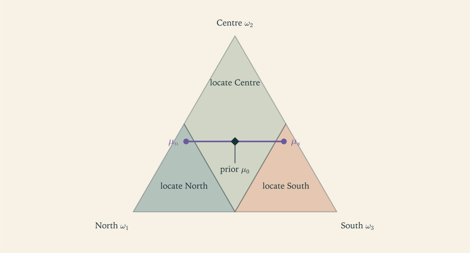
A distributor must place its single regional warehouse in the North, the Centre, or the South, three towns equally spaced along one highway. Demand this season will be concentrated in one of the three towns; call these states \(\omega_1\) (North), \(\omega_2\) (Centre), \(\omega_3\) (South). Shipping costs one unit per segment of highway, so with positions \(0,1,2\) the payoff of locating at town \(a\) when demand is at town \(\omega\) is minus the distance between them. A belief is a vector \((\mu(\omega_1),\mu(\omega_2),\mu(\omega_3))\) , and the three affine functions are

\[ \ell_N(\mu)=-\mu(\omega_2)-2\mu(\omega_3),\qquad \ell_C(\mu)=-\mu(\omega_1)-\mu(\omega_3),\qquad \ell_S(\mu)=-2\mu(\omega_1)-\mu(\omega_2). \]

Comparing them pairwise, \(\ell_N\ge\ell_C\) if and only if \(\mu(\omega_1)\ge\mu(\omega_2)+\mu(\omega_3)\) , that is \(\mu(\omega_1)\ge\tfrac12\) , and \(\ell_N\ge\ell_S\) if and only if \(\mu(\omega_1)\ge\mu(\omega_3)\) , which follows from the first. By symmetry,

\[ R(N)=\{\mu:\mu(\omega_1)\ge\tfrac12\},\qquad R(S)=\{\mu:\mu(\omega_3)\ge\tfrac12\},\qquad R(C)=\{\mu:\mu(\omega_1)\le\tfrac12,\ \mu(\omega_3)\le\tfrac12\}. \]

The best location is a median of the belief, the familiar rule for absolute-distance loss. The regions are two corner triangles and a central quadrilateral; all three meet only at the belief \((\tfrac12,0,\tfrac12)\) , where every location costs \(1\) in expectation.

Let the prior be \(\mu_0=(\tfrac{3}{10},\tfrac25,\tfrac{3}{10})\) . Its median is the Centre, and \(U(\mu_0)=-\tfrac35\) . A survey of retailers returns \(n\) (northern) with probability \(\tfrac{9}{10}\) , \(\tfrac12\) , \(\tfrac{1}{10}\) in the three states and \(s\) (southern) otherwise. Then \(\pi(n)=\tfrac{27}{100}+\tfrac{20}{100}+\tfrac{3}{100}=\tfrac12\) and

\[ \mu_n=\bigl(\tfrac{27}{50},\tfrac25,\tfrac{3}{50}\bigr),\qquad \mu_s=\bigl(\tfrac{3}{50},\tfrac25,\tfrac{27}{50}\bigr). \]

After \(n\) the North is the median, since \(\tfrac{27}{50}\ge\tfrac12\) , and \(U(\mu_n)=\ell_N(\mu_n)=-\tfrac25-\tfrac{6}{50}=-\tfrac{13}{25}\) ; after \(s\) the South is chosen with the same value by symmetry. The survey raises the expected payoff from \(-\tfrac35\) to \(-\tfrac{13}{25}\) , a value of information of \(\tfrac{2}{25}\) . The gain is small because both posteriors land just inside the corner regions; a survey whose posteriors stayed inside the central region would be worth nothing, however much it moved beliefs.

2.2 What an experiment is worth

Now attach an experiment. An experiment \(\pi=(S,\{\pi(\cdot\mid\omega)\}_{\omega\in\Omega})\) (Definition 1.1) has finitely many realizations. Following the course’s default convention, the prior \(\mu_0\) has full support throughout this chapter; Definition 1.1 itself does not require it, but the converse half of Blackwell’s theorem below does. Realization \(s\) has probability \(\pi(s)=\sum_\omega\mu_0(\omega)\pi(s\mid\omega)\) , and when \(\pi(s)>0\) the posterior is \(\mu_s(\omega)=\mu_0(\omega)\pi(s\mid\omega)/\pi(s)\) (math.probability-theory.bayes-rule). The decision maker observes \(s\) and then acts. A decision rule tells her what to do after each realization, possibly at random; write \(\delta(a\mid s)\) for the probability of action \(a\) after \(s\) , with each \(\delta(\cdot\mid s)\) supported on finitely many actions. The value of information is the gain from the best rule over acting on the prior alone,

and the first part of the next proposition justifies writing the best rule’s payoff as \(E_{\tau_\pi}[U(\mu)]\) .

Part (a) settles the promise made in Chapter 1. The realizations of an experiment are labels; what the decision maker can do with them depends only on the beliefs they produce and how often they produce them. Relabelling realizations, merging two realizations that produce the same posterior, or splitting one realization into two copies by a coin flip all leave \(\tau_\pi\) , and therefore every value, unchanged.

Part (b) is often stated as Jensen’s inequality: \(U\) is convex and \(E_{\tau_\pi}[\mu]=\mu_0\) , so \(E_{\tau_\pi}[U(\mu)]\ge U(E_{\tau_\pi}[\mu])\) . The proof above uses only a supporting line of \(U\) at the prior, namely \(\ell_{a_0}\) , and it pays for its directness with an exact formula. The value of information is the expected amount by which the best action at the realized posterior beats the action that would have been chosen at the prior, measured at that posterior. Information is worthless exactly when it never changes what is optimal, and in that case the prior-optimal action stays optimal everywhere the experiment can lead.

2.3 Garbling: noise added after the fact

The comparison problem needs a notion of “more informative” that does not refer to any decision. The natural one is operational. If the realization of \(\pi'\) can be produced by taking the realization of \(\pi\) and passing it through a random device that does not look at the state, then anyone holding \(\pi\) can simulate \(\pi'\) , and \(\pi'\) cannot be more useful.

In matrix language, let \(P\) be the \(n\times\lvert S\rvert\) matrix with entries \(P_{\omega s}=\pi(s\mid\omega)\) , whose rows are probability vectors, and similarly \(P'\) for \(\pi'\) . A Markov kernel is a \(\lvert S\rvert\times\lvert S'\rvert\) row-stochastic matrix \(G\) , and garbling says \(P'=PG\) . The kernel acts on realizations, and the crucial restriction is that it is the same in every state: the noise is added by someone who does not know \(\omega\) . A device allowed to depend on the state could manufacture information from nothing.

Three garblings are always available. Every experiment is a garbling of full disclosure \(\bar\pi\) , whose realization is the state itself: take \(g(s\mid\omega)=\pi(s\mid\omega)\) . No disclosure \(\underline\pi\) , with a single realization, is a garbling of every experiment: send every realization to it. And every experiment is a garbling of itself, by the identity kernel. Composing two kernels gives a kernel, so the relation \(\succeq\) is reflexive and transitive. It is not antisymmetric, because an experiment and a copy of it with one realization split into two by a coin flip are garblings of each other; Exercise 2.4 asks for the details and for what such pairs have in common.

Finding a kernel is a linear feasibility problem: the unknowns \(g(s'\mid s)\) enter the defining equations linearly, together with the constraints of nonnegativity and unit row sums. For small experiments it can be solved by hand.

2.4 Blackwell’s theorem

We can now state the theorem that ties the three notions together. Condition (iii) needs a name for the spreading seen in Example 2.4. A distribution of posteriors \(\tau\) is a mean-preserving spread of \(\tau'\) if each posterior of \(\tau'\) can be split into posteriors of \(\tau\) that average back to it, in proportions that reproduce \(\tau\) .

Before the proof, notice what is and is not surprising. That (i) implies (ii) is the simulation argument from the start of Section 2.3: a decision maker who sees \(s\) can draw \(s'\) from \(g(\cdot\mid s)\) herself and then use any rule designed for \(\pi'\) , so she can do at least as well with \(\pi\) . That (iii) implies (iv) is Jensen’s inequality applied posterior by posterior, and that (iv) implies (ii) is Proposition 2.2. The surprise is the converse: an experiment that is weakly better for every decision maker can always be degraded into the other by state-independent noise. Nothing in (ii) mentions kernels, and the kernel must be produced from a family of inequalities about payoffs. That step needs one result from linear programming, which we import with its hypotheses.

The imported result. A linear program in standard form is “minimize \(c^{\top}z\) subject to \(Mz=b\) and \(z\ge 0\) ”, with \(z\in\mathbb R^p\) and \(M\) an \(m\times p\) matrix of full row rank \(m\) , and its dual is “maximize \(b^{\top}\eta\) subject to \(M^{\top}\eta\le c\) ”, with \(\eta\in\mathbb R^m\) unrestricted in sign. Two facts are needed. First, if the standard-form program is feasible and its objective is bounded below on the feasible set, then it has an optimal solution. Second, strong duality: if the standard-form program has an optimal solution, then its dual has an optimal solution and the two optimal values are equal. In Continuous Optimization the second is Theorem 4.10 and the first is the remark that follows its proof; both rest on the termination of the simplex method under Bland’s rule, which that course states without proof, and both assume the full-rank hypothesis (math.continuous-optimization.linear-programming-vertices-duality).

Read the last step again with the dual variables in mind. The certificate that no kernel exists is a vector \(\lambda\) indexed by states and realizations of \(\pi'\) , and dividing by the prior turns it into a payoff table. The constraint \(\sum_\omega\pi(s\mid\omega)\lambda(\omega,s')+\kappa(s)\le 0\) says that, after any realization of \(\pi\) , no action earns more than \(-\kappa(s)\) ; the dual objective says that obeying \(\pi'\) earns more than all of these bounds together. The certificate is a decision maker who prefers \(\pi'\) . The same mechanism appears in Game Theory, where a pure strategy is never a best response exactly when it is strictly dominated by a mixed strategy (Game Theory, Proposition 4.6); that course proves it with the minimax theorem (its Theorem 4.4), itself a consequence of linear-programming duality, so that the failure of one system of inequalities produces a solution of another.

Three consequences are worth stating. First, the proof uses decision problems with at most \(\lvert S'\rvert\) actions and bounded payoffs, so (ii) may be weakened to that class without changing the theorem. Second, condition (i) does not mention the prior. Hence if \(\pi\) is weakly better than \(\pi'\) in every decision problem at one full-support prior, it is so at every full-support prior; a ranking in a single decision problem, by contrast, can reverse when the prior moves (Exercise 2.10). Third, the step from (i) to (iii) is worth isolating because later chapters lean on it: a garbling produces a mean-preserving contraction of posteriors. Applying any linear map to the beliefs preserves the averaging, so it also produces a mean-preserving contraction of any posterior expectation, such as the posterior mean \(E_\mu[\omega]\) of a real-valued state. Chapter 8 builds mean-based persuasion on exactly this fact.

The theorem also yields a quick screening test. By (iii), every posterior of a garbling of \(\pi\) lies in the convex hull of the posteriors of \(\pi\) . In Example 2.4 the posterior \(\tfrac{13}{14}\) of \(\pi''\) lies outside the interval \([\tfrac17,\tfrac67]\) spanned by the posteriors of \(\pi\) , so \(\pi''\) could not have been a garbling, and the decision problem found there acts precisely on the part of the belief space that \(\pi\) never reaches.

2.5 Forecasts that cannot be ranked

Blackwell’s order is partial. Most pairs of experiments are not comparable, and for those the opening question has the answer no: each is strictly better for some decision maker. With a binary state the comparison reduces to a family of one-dimensional functions that can be drawn.

The functions \((\mu-k)^+\) are the payoffs of call options on the posterior, and each is itself the value of a two-action decision problem: act, earning \(\omega-k\) , or do nothing, earning \(0\) . So with a binary state, Blackwell’s order is decided by two-action problems alone: if \(\pi\) is weakly better in every two-action problem, it is weakly better for every call, and Corollary 2.6 applies. Exercise 2.7 proves the converse description, that every two-action problem is a call plus affine terms. The map \(k\mapsto E_\tau[(\mu-k)^+]\) equals \(\int_k^1\Pr_\tau(\mu>x)\,dx\) , and the one-dimensional case of the equivalence of (iii) and (iv) in Theorem 2.5 is the characterization of increasing risk by Rothschild and Stiglitz (1970), stated there for random variables with a common mean rather than for experiments.

Example 2.6: The two forecasts, compared for every margin

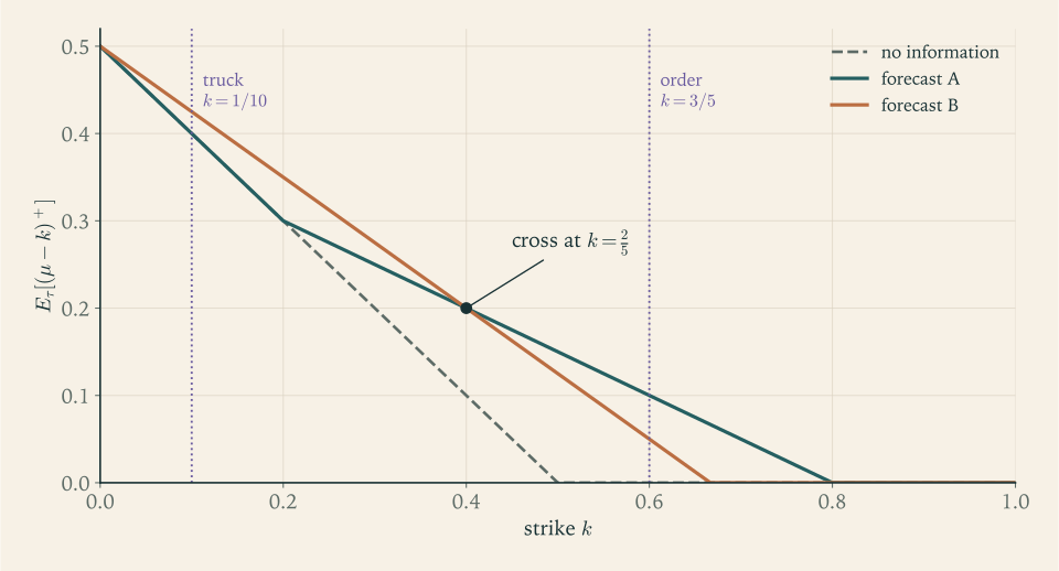
Take forecasts A and B of Example 2.3 at \(\mu_0=\tfrac12\) . Forecast A puts probability \(\tfrac12\) on each of the posteriors \(\tfrac15\) and \(\tfrac45\) ; forecast B puts \(\tfrac14\) on \(0\) and \(\tfrac34\) on \(\tfrac23\) . The call functions are piecewise linear:

\[ E_{\tau_A}\bigl[(\mu-k)^+\bigr]=\begin{cases}\tfrac12-k,&0\le k\le\tfrac15,\\ \tfrac25-\tfrac k2,&\tfrac15\le k\le\tfrac45,\\ 0,&k\ge\tfrac45,\end{cases}\qquad E_{\tau_B}\bigl[(\mu-k)^+\bigr]=\begin{cases}\tfrac12-\tfrac{3k}{4},&0\le k\le\tfrac23,\\ 0,&k\ge\tfrac23.\end{cases} \]

On \([\tfrac15,\tfrac23]\) the difference B minus A is \(\tfrac{1}{10}-\tfrac k4\) , which changes sign at \(k=\tfrac25\) . For \(k<\tfrac25\) forecast B gives the larger value, and for \(\tfrac25<k<\tfrac45\) forecast A does. Neither inequality of Corollary 2.6 holds for all \(k\) , so neither forecast is a garbling of the other.

The newsvendor of Example 2.3 had \(U(\mu)=400+600(\mu-\tfrac35)^+\) , a call at \(k=\tfrac35\) , where A wins: \(600\cdot(\tfrac25-\tfrac{3}{10})=60\) against \(600\cdot(\tfrac12-\tfrac{9}{20})=30\) , the two values computed there. Now take a different decision with a low threshold. The retailer can reserve a backup truck for 1 dollar per unit of capacity, and the reservation saves 10 dollars per unit if demand is high. Reserving earns \(10\mu-1\) in expectation, so \(U(\mu)=10(\mu-\tfrac{1}{10})^+\) . At the prior, \(U(\tfrac12)=4\) . Forecast A leaves both posteriors above \(\tfrac{1}{10}\) , so the retailer reserves after either report and gains nothing: \(E_{\tau_A}[(\mu-\tfrac{1}{10})^+]=\tfrac12\cdot\tfrac{7}{10}+\tfrac12\cdot\tfrac{1}{10}=\tfrac25\) , which equals \((\tfrac12-\tfrac{1}{10})^+\) , so \(\mathrm{VOI}(\pi_A)=0\) . Forecast B identifies some low seasons for certain, and

\[ \mathrm{VOI}(\pi_B)=10\Bigl(\tfrac34\bigl(\tfrac23-\tfrac{1}{10}\bigr)-\tfrac25\Bigr)=10\Bigl(\tfrac{17}{40}-\tfrac{16}{40}\Bigr)=\tfrac14 . \]

For the truck decision, A is worthless and B is worth a quarter of a dollar per unit. That settles the opening question: the retailer cannot rank the forecasts without knowing which decisions they will serve.

Common mistake. Ranking experiments by a single summary of their likelihoods: the number of realizations, the probability of a correct report, or the accuracy in one state. Forecast A is correct with probability \(\tfrac45\) and forecast B with probability \(\tfrac34\) , yet B is better for the truck decision; forecast B is perfect in high seasons, yet A is better for the order decision. Adding realizations does not help either, as Example 2.4 already showed: the three-realization experiment \(\pi\) there was beaten by the two-realization \(\pi''\) in a decision problem that pays only at very confident beliefs. The repair is to compare whole distributions of posteriors, by a kernel, by Corollary 2.6 when the state is binary, or by exhibiting decision problems that rank the experiments in opposite directions.

2.6 Quadratic loss sees only the posterior mean

One family of decision problems has a closed-form value of information that applied work uses constantly. Let the state be a real number, so that \(\Omega\subset\mathbb R\) is a finite set of values, and let the decision maker estimate it under quadratic loss: \(A=\mathbb R\) and \(u(a,\omega)=-(a-\omega)^2\) . Write \(m=E_\mu[\omega]\) for the posterior mean, \(m_0=E_{\mu_0}[\omega]\) for the prior mean, and \(\operatorname{Var}_\mu(\omega)=E_\mu[(\omega-m)^2]\) .

The identity is the law of total variance read as a statement about decisions: prior variance splits into the expected posterior variance, which is the loss that remains, and the variance of the posterior mean, which is the loss that information removes (math.probability-theory.tower-property). Note that \(U(\mu)=-E_\mu[\omega^2]+(E_\mu[\omega])^2\) is convex in \(\mu\) , as Proposition 2.2 says it must be: a linear term plus the square of a linear term.

Proposition 2.7 is convenient and dangerous. It compresses an experiment into one number, and a single number cannot carry a partial order.

2.7 What the comparison of experiments became

The comparison of experiments has a short prehistory. Bohnenblust, Shapley, and Sherman (1949, RAND memorandum) compared experiments through the decision problems they serve, and Blackwell (1951, 1953) then proved the comparison theorem in the language of statistical experiments, where a statistician chooses which observations to collect before facing an estimation or testing problem; the finite case proved here contains its main ideas. Crémer (1982) gave a short proof of the hard direction by linear programming, in the spirit of the one above. Le Cam (1964) quantified the comparison: the deficiency of one experiment relative to another measures how far it is from being obtainable by garbling the other, a one-sided quantity, and the larger of the two deficiencies defines a distance between experiments. In economics the theorem became the standard meaning of “more information”: Marschak and Miyasawa (1968) used it to compare information systems for organizations. Through Rothschild and Stiglitz (1970), discussed after Corollary 2.6, the spreading condition also became the standard language for comparing risky prospects.

The order’s main weakness is visible in Example 2.6: it is very incomplete. Two responses shaped the literature. One restricts the class of decision problems. Lehmann (1988) compared experiments for monotone decision problems, in which higher states favour higher actions, among experiments whose likelihoods satisfy a monotone likelihood ratio property; this ranks many more pairs, and it is the order used when firms or bidders acquire information about a one-dimensional state. The other response keeps all decision problems but looks at a single summary, as in Section 2.6, accepting that it ranks experiments only for one decision. A separate line, begun by Radner and Stiglitz (1984), studied the value of information as a function of a parameter that indexes how much is acquired and found the nonconcavity seen in the accuracy family after Example 2.3.

For this course the theorem matters in three places. Chapter 6 replaces the decision maker by a sender whose value from the receiver’s belief, \(\hat v\) , is not convex. Proposition 2.3 then fails: the sender can lose from information, and choosing the information optimally becomes a problem of taking the concave envelope of \(\hat v\) , the mirror image of the convexity used here. Kamenica and Gentzkow (2011) built that theory on the description of experiments by distributions of posteriors, and Gentzkow and Kamenica (2016) used the step “garbling yields a mean-preserving contraction” to characterize the distributions of posterior means a designer can induce, which is the starting point of Chapter 8. Chapter 9 turns to games, where Proposition 2.3 can fail even for players who receive the information themselves, because the information also changes how others act. Bergemann and Morris (2016) observe that information then plays two roles: it makes more outcomes feasible, and it imposes more incentive constraints, since a better-informed player has more ways to deviate. Their many-player extension of Blackwell’s order, individual sufficiency, is exactly the order under which more information shrinks the set of Bayes correlated equilibria, so one order captures both roles.

A question to carry forward: in Example 2.1 the shop, left alone, values the test at \(\tfrac{5}{12}\) . If the test were designed by the item’s supplier, who earns a commission whenever the shop stocks, which test would the supplier choose, and would the shop still be glad to see it? Chapter 6 answers both.

Exercises

1. State Definition 2.4 and the four conditions of Theorem 2.5 from memory, and for each of the four implications proved in Section 2.4 name the one tool it consumes: Bayes’ rule, Jensen’s inequality, convexity of \(U\) , or linear-programming duality.

   Hint

   Garbling: a Markov kernel \(g(s'\mid s)\) , the same in every state, with \(\pi'(s'\mid\omega)=\sum_sg(s'\mid s)\pi(s\mid\omega)\) . The four conditions are garbling, every decision maker weakly prefers \(\pi\) , mean-preserving spread, and the inequality for every convex \(\varphi\) . In the proof, (i) to (iii) consumes Bayes’ rule (each posterior of \(\pi'\) is an average of posteriors of \(\pi\) ); (iii) to (iv) consumes Jensen’s inequality; (iv) to (ii) consumes the convexity of \(U\) from Proposition 2.2; (ii) to (i) consumes linear-programming duality, whose dual solution becomes the payoff table.

2. A loan officer with \(\Omega=\{0,1\}\) and prior \(\mu_0=\tfrac14\) can approve, earning \(2\) if the borrower repays (\(\omega=1\) ) and losing \(1\) otherwise, or reject for \(0\) ; a credit test reports \(h\) with probability \(\tfrac45\) if \(\omega=1\) and \(\tfrac15\) if \(\omega=0\) . Find \(U\) , the approval threshold, both posteriors, \(\mathrm{VOI}\) , and the largest fee the officer would pay for the test.

   Solution

   Identify a belief with \(\mu=\Pr(\omega=1)\) . Approving earns \(\ell_1(\mu)=2\mu-(1-\mu)=3\mu-1\) and rejecting earns \(0\) , so

   \[ U(\mu)=\max\{0,\,3\mu-1\}, \]

   and the officer approves exactly when \(\mu\ge\tfrac13\) . At the prior \(\mu_0=\tfrac14\) she rejects and \(U(\mu_0)=0\) .

   The test reports \(h\) with probability

   \[ \pi(h)=\tfrac14\cdot\tfrac45+\tfrac34\cdot\tfrac15=\tfrac15+\tfrac{3}{20}=\tfrac{7}{20}, \]

   so the posteriors are

   \[ \mu_h=\frac{1/5}{7/20}=\tfrac47,\qquad \mu_l=\frac{\tfrac14\cdot\tfrac15}{13/20}=\tfrac{1}{13}. \]

   They average to the prior: \(\tfrac{7}{20}\cdot\tfrac47+\tfrac{13}{20}\cdot\tfrac{1}{13}=\tfrac15+\tfrac{1}{20}=\tfrac14\) . After \(h\) the posterior \(\tfrac47\) exceeds the threshold, so she approves and expects \(U(\tfrac47)=\tfrac{12}{7}-1=\tfrac57\) ; after \(l\) she rejects. By Proposition 2.3(a),

   \[ \mathrm{VOI}(\pi)=\tfrac{7}{20}\cdot\tfrac57+\tfrac{13}{20}\cdot 0-0=\tfrac14 . \]

   Directly: approving after \(h\) earns \(2\) on the event \(\{\omega=1,h\}\) of probability \(\tfrac15\) and loses \(1\) on \(\{\omega=0,h\}\) of probability \(\tfrac{3}{20}\) , for \(\tfrac25-\tfrac{3}{20}=\tfrac14\) . The largest fee the officer would pay is therefore \(\tfrac14\) : at any lower fee buying the test raises her expected payoff, and at a higher fee it lowers it.

3. Write explicit Markov kernels showing that every experiment \(\pi\) is a garbling of full disclosure \(\bar\pi\) and that no disclosure \(\underline\pi\) is a garbling of \(\pi\) , and prove that \(\mathrm{VOI}(\bar\pi)=E_{\mu_0}\bigl[\max_{a}u(a,\omega)\bigr]-U(\mu_0)\) , the expected value of perfect information.

   Solution

   Full disclosure. The experiment \(\bar\pi\) has realization set \(\Omega\) and \(\bar\pi(\omega'\mid\omega)=\mathbf 1\{\omega'=\omega\}\) . Given any \(\pi\) on \(S\) , define the kernel from \(\Omega\) to \(S\) by \(g(s\mid\omega')=\pi(s\mid\omega')\) ; its rows are probability vectors. Then

   \[ \sum_{\omega'}g(s\mid\omega')\,\bar\pi(\omega'\mid\omega)=g(s\mid\omega)=\pi(s\mid\omega), \]

   so \(\pi\) is a garbling of \(\bar\pi\) : whoever knows the state can simulate any experiment by running it herself.

   No disclosure. The experiment \(\underline\pi\) has one realization \(s_\varnothing\) with \(\underline\pi(s_\varnothing\mid\omega)=1\) . The kernel \(g(s_\varnothing\mid s)=1\) for every \(s\in S\) gives \(\sum_sg(s_\varnothing\mid s)\pi(s\mid\omega)=1\) , so \(\underline\pi\) is a garbling of \(\pi\) .

   Value of full disclosure. The posterior after realization \(\omega\) is the vertex \(e_\omega\) of the simplex, the point mass on \(\omega\) , which occurs with probability \(\mu_0(\omega)\) , so \(\tau_{\bar\pi}(e_\omega)=\mu_0(\omega)\) . At a vertex, \(U(e_\omega)=\max_au(a,\omega)\) . By Proposition 2.3(a),

   \[ \mathrm{VOI}(\bar\pi)=\sum_\omega\mu_0(\omega)\max_au(a,\omega)-U(\mu_0)=E_{\mu_0}\bigl[\max_au(a,\omega)\bigr]-U(\mu_0). \]

   By Theorem 2.5 this is the largest value any experiment can have in this decision problem, since every experiment is a garbling of \(\bar\pi\) .

4. Show that the Blackwell order is reflexive and transitive by composing kernels, then give two experiments with different numbers of realizations, each a garbling of the other, and say what their distributions of posteriors must have in common.

   Answer

   Reflexive: the identity kernel \(g(s'\mid s)=\mathbf 1\{s'=s\}\) . Transitive: if \(\pi'=\pi\) garbled by \(g\) and \(\pi''=\pi'\) garbled by \(g'\) , then \(g''(s''\mid s)=\sum_{s'}g'(s''\mid s')g(s'\mid s)\) is a kernel and carries \(\pi\) to \(\pi''\) . Not antisymmetric: let \(\pi\) have realizations \(h,l\) and let \(\tilde\pi\) split \(h\) into \(h_1,h_2\) with \(\tilde\pi(h_1\mid\omega)=\tilde\pi(h_2\mid\omega)=\tfrac12\pi(h\mid\omega)\) ; merging \(h_1,h_2\) into \(h\) , and splitting \(h\) by a fair coin, are kernels in the two directions. Mutual garblings always have the same distribution of posteriors: applying (iv) of Theorem 2.5 in both directions to the strictly convex \(\varphi(\mu)=\sum_\omega\mu(\omega)^2\) gives equality in Jensen’s inequality, which forces each \(K(\cdot\mid\mu')\) to sit on \(\mu'\) , so \(\tau_\pi=\tau_{\tilde\pi}\) .

5. A consultant argues that an experiment with three realizations is at least as informative as one with two. With \(\Omega=\{0,1\}\) and \(\mu_0=\tfrac12\) , let \(\pi(\cdot\mid 1)=(\tfrac12,\tfrac14,\tfrac14)\) and \(\pi(\cdot\mid 0)=(\tfrac14,\tfrac14,\tfrac12)\) , and let \(\pi'(h\mid 1)=\tfrac{9}{10}\) and \(\pi'(h\mid 0)=\tfrac{1}{10}\) ; find a decision problem in which \(\pi'\) is strictly better and name the flaw in the argument.

   Solution

   At \(\mu_0=\tfrac12\) the realizations of \(\pi\) have probabilities \(\tfrac38,\tfrac14,\tfrac38\) and posteriors

   \[ \mu_{s_1}=\frac{1/4}{3/8}=\tfrac23,\qquad \mu_{s_2}=\tfrac12,\qquad \mu_{s_3}=\frac{1/8}{3/8}=\tfrac13 . \]

   The realizations of \(\pi'\) each have probability \(\tfrac12\) , with posteriors \(\tfrac{9}{10}\) and \(\tfrac{1}{10}\) . Take a decision problem that rewards confidence: an action paying \(\tfrac15\) if \(\omega=1\) and \(-\tfrac45\) if \(\omega=0\) , against a safe action paying \(0\) . Then \(U(\mu)=(\mu-\tfrac45)^+\) and \(U(\mu_0)=0\) . Every posterior of \(\pi\) is at most \(\tfrac23<\tfrac45\) , so \(\mathrm{VOI}(\pi)=0\) , while

   \[ \mathrm{VOI}(\pi')=\tfrac12\Bigl(\tfrac{9}{10}-\tfrac45\Bigr)=\tfrac{1}{20}>0 . \]

   The flaw is to treat the number of realizations as a measure of information. Realizations are labels; what matters is the distribution of posteriors they produce (Proposition 2.3(a)). Here the middle realization of \(\pi\) leaves the belief at the prior, and the other two are less decisive than those of \(\pi'\) . In fact \(\pi\) is a garbling of \(\pi'\) : the kernel \(g(s_1\mid h)=\tfrac{17}{32}\) , \(g(s_2\mid h)=\tfrac14\) , \(g(s_3\mid h)=\tfrac{7}{32}\) , \(g(s_1\mid l)=\tfrac{7}{32}\) , \(g(s_2\mid l)=\tfrac14\) , \(g(s_3\mid l)=\tfrac{17}{32}\) reproduces \(\pi\) , as one checks state by state, so the two-realization experiment is the more informative one.

6. In Example 2.2, use the splitting lemma (Theorem 1.4) to build an experiment with two equally likely posteriors on the boundary of \(R(C)\) , one with \(\mu(\omega_1)=\tfrac12\) and one with \(\mu(\omega_3)=\tfrac12\) , so that a distributor who breaks ties away from the Centre always relocates; show the experiment is worthless, and find the value of the experiment whose posteriors are \((\tfrac12+\varepsilon,\tfrac25,\tfrac{1}{10}-\varepsilon)\) and its mirror image, for \(0\le\varepsilon\le\tfrac{1}{10}\) .

   Solution

   In Example 2.2 the Centre is optimal exactly on \(R(C)=\{\mu:\mu(\omega_1)\le\tfrac12,\ \mu(\omega_3)\le\tfrac12\}\) , and the prior is \(\mu_0=(\tfrac{3}{10},\tfrac25,\tfrac{3}{10})\) . Look for two equally likely posteriors, symmetric under exchanging North and South, of the form \((\tfrac12,x,\tfrac12-x)\) and \((\tfrac12-x,x,\tfrac12)\) . Their average is \((\tfrac12-\tfrac x2,x,\tfrac12-\tfrac x2)\) , which equals the prior when \(x=\tfrac25\) . So the posteriors are

   \[ \mu_n=\bigl(\tfrac12,\tfrac25,\tfrac{1}{10}\bigr),\qquad \mu_s=\bigl(\tfrac{1}{10},\tfrac25,\tfrac12\bigr), \]

   and the splitting lemma gives \(\pi(n\mid\omega)=\tfrac12\mu_n(\omega)/\mu_0(\omega)\) , that is

   \[ \pi(n\mid\omega_1)=\tfrac56,\qquad \pi(n\mid\omega_2)=\tfrac12,\qquad \pi(n\mid\omega_3)=\tfrac16 . \]

   At \(\mu_n\) the North and the Centre tie: \(\ell_N(\mu_n)=-\tfrac25-\tfrac15=-\tfrac35=\ell_C(\mu_n)\) . So a distributor who breaks ties away from the Centre moves the warehouse after every realization, yet the Centre, optimal at the prior, is still optimal at both posteriors, and by Proposition 2.3(c) the experiment is worth exactly \(0\) .

   Now push the posteriors to \((\tfrac12+\varepsilon,\tfrac25,\tfrac{1}{10}-\varepsilon)\) and its mirror image; they still average to \(\mu_0\) . At the first, \(\ell_N=-\tfrac25-2(\tfrac{1}{10}-\varepsilon)=-\tfrac35+2\varepsilon\) , while \(\ell_C=-(\tfrac12+\varepsilon)-(\tfrac{1}{10}-\varepsilon)=-\tfrac35\) and \(\ell_S\) is lower still. By symmetry the same holds at the mirror posterior, so

   \[ \mathrm{VOI}=\bigl(-\tfrac35+2\varepsilon\bigr)-\bigl(-\tfrac35\bigr)=2\varepsilon . \]

   The value grows linearly from zero as the posteriors leave \(R(C)\) : what matters is how far the posteriors cross the boundary, not whether the chosen location changes.

7. For a binary state and any decision problem with two actions, show that \(U(\mu)=\alpha+\beta\mu+c(\mu-k)^+\) for some numbers \(\alpha,\beta\) , some \(c\ge 0\) , and some \(k\in[0,1]\) , deduce that \(\mathrm{VOI}(\pi)=c\bigl(E_{\tau_\pi}[(\mu-k)^+]-(\mu_0-k)^+\bigr)\) , and conclude with Corollary 2.6 that two-action problems suffice to test the Blackwell order.

   Solution

   With two actions \(a,b\) and a binary state, each \(\ell_x(\mu)=u(x,0)+\mu\bigl(u(x,1)-u(x,0)\bigr)\) is affine, and

   \[ U=\max\{\ell_a,\ell_b\}=\ell_b+(\ell_a-\ell_b)^+ . \]

   Write \(\ell_a-\ell_b=d_0+(d_1-d_0)\mu\) with \(d_\omega=u(a,\omega)-u(b,\omega)\) . If \(d_1=d_0\) the difference is constant and \(U\) is affine. If \(d_1>d_0\) , put \(k=d_0/(d_0-d_1)\) , so that \(\ell_a-\ell_b=(d_1-d_0)(\mu-k)\) and \((\ell_a-\ell_b)^+=(d_1-d_0)(\mu-k)^+\) . If \(d_1<d_0\) , then \((\ell_a-\ell_b)^+=(d_0-d_1)(k-\mu)^+=(d_0-d_1)\bigl[(\mu-k)^+-(\mu-k)\bigr]\) , again an affine function plus a nonnegative multiple of \((\mu-k)^+\) . If \(k\) falls outside \([0,1]\) , \((\mu-k)^+\) is affine on \([0,1]\) and \(U\) is affine there. In all cases \(U(\mu)=\alpha+\beta\mu+c(\mu-k)^+\) with \(c\ge 0\) and \(k\in[0,1]\) , or \(U\) is affine.

   Affine terms have the same expectation under \(\tau_\pi\) as at \(\mu_0\) by Bayes plausibility, so

   \[ \mathrm{VOI}(\pi)=c\Bigl(E_{\tau_\pi}\bigl[(\mu-k)^+\bigr]-(\mu_0-k)^+\Bigr). \]

   Conversely, each call \((\mu-k)^+\) with \(k\in[0,1]\) is the value of the two-action problem in which one action pays \(\omega-k\) and the other pays \(0\) . Hence \(\pi\) is weakly better than \(\pi'\) in every two-action problem if and only if the inequality of Corollary 2.6 holds for every \(k\) , which by that corollary is equivalent to \(\pi\succeq\pi'\) .

8. In Example 2.2 replace the noisy survey by one that reveals only whether demand is in the South; compute its posteriors, the chosen locations, and its value of information, then exhibit a decision problem in which the noisy survey is strictly more valuable, so that the two surveys are Blackwell incomparable.

   Solution

   The South survey reveals whether \(\omega=\omega_3\) . With \(\mu_0=(\tfrac{3}{10},\tfrac25,\tfrac{3}{10})\) , the report “South” has probability \(\tfrac{3}{10}\) and posterior \((0,0,1)\) , where the South is the median and \(U=0\) . The report “not South” has probability \(\tfrac{7}{10}\) and posterior

   \[ \bigl(\tfrac37,\tfrac47,0\bigr), \]

   whose median is the Centre because \(\tfrac37\le\tfrac12\) and \(0\le\tfrac12\) ; there \(U=\ell_C=-\tfrac37-0=-\tfrac37\) . The expected payoff with the survey is \(\tfrac{7}{10}\cdot(-\tfrac37)=-\tfrac{3}{10}\) , so

   \[ \mathrm{VOI}=-\tfrac{3}{10}+\tfrac35=\tfrac{3}{10}, \]

   much more than the \(\tfrac{2}{25}\) of the noisy survey: whenever demand is in the South, which has probability \(\tfrac{3}{10}\) , the survey moves the warehouse there from the Centre and saves one segment of highway.

   For the reverse ranking, consider a bet on the North that pays \(1\) if \(\omega=\omega_1\) and \(-1\) otherwise, against not betting for \(0\) . Then \(U(\mu)=\max\{0,2\mu(\omega_1)-1\}\) , and the prior gives \(0\) . The noisy survey produces \(\mu_n(\omega_1)=\tfrac{27}{50}\) with probability \(\tfrac12\) , worth \(2\cdot\tfrac{27}{50}-1=\tfrac{2}{25}\) , and \(\mu_s(\omega_1)=\tfrac{3}{50}\) , worth \(0\) , so its value is \(\tfrac{1}{25}\) . The South survey leaves \(\mu(\omega_1)\) at \(0\) or \(\tfrac37\) , both below \(\tfrac12\) , so its value is \(0\) . Each survey is strictly better in one decision problem, so by Theorem 2.5, (i) implies (ii), neither is a garbling of the other.

9. Let \(\pi\) have realizations \(s_1,s_2,s_3\) with \(\pi(\cdot\mid 1)=(\tfrac12,\tfrac12,0)\) and \(\pi(\cdot\mid 0)=(0,\tfrac12,\tfrac12)\) , and let \(\pi'\) report \(h\) with probability \(\tfrac23\) when \(\omega=1\) and \(\tfrac13\) when \(\omega=0\) ; find every Markov kernel that carries \(\pi\) to \(\pi'\) and explain why a garbling kernel need not be unique.

   Solution

   Write \(x_j=g(h\mid s_j)\) ; then \(g(l\mid s_j)=1-x_j\) and the unit row sums hold automatically. The defining equations for the realization \(h\) are

   \[ \tfrac12x_1+\tfrac12x_2=\tfrac23\quad(\omega=1),\qquad \tfrac12x_2+\tfrac12x_3=\tfrac13\quad(\omega=0), \]

   and those for \(l\) follow from them because the likelihoods of both experiments sum to one in each state. Put \(x_2=t\) . Then \(x_1=\tfrac43-t\) and \(x_3=\tfrac23-t\) . The bounds \(0\le x_j\le 1\) require \(t\ge\tfrac13\) (from \(x_1\le 1\) ), \(t\le\tfrac23\) (from \(x_3\ge 0\) ), and \(0\le t\le 1\) . So the kernels are exactly

   \[ g(h\mid s_1)=\tfrac43-t,\qquad g(h\mid s_2)=t,\qquad g(h\mid s_3)=\tfrac23-t,\qquad t\in\bigl[\tfrac13,\tfrac23\bigr]. \]

   For instance \(t=\tfrac12\) gives \((\tfrac56,\tfrac12,\tfrac16)\) . The kernel is not unique because the realization \(s_2\) is equally likely in both states: it carries no information, so it may be sent to \(h\) with any probability \(t\) , and the informative realizations \(s_1\) and \(s_3\) adjust to keep the two state-by-state likelihoods of \(h\) correct. There are two equations and three unknowns, and the feasible set is a segment.

10. Prove from Theorem 2.5 that if \(\pi\) is weakly more valuable than \(\pi'\) in every decision problem at one full-support prior, then it is so at every full-support prior; then use forecasts A and B in the order problem of Example 2.3 to show that a ranking in one decision problem can reverse when the prior changes.

    Solution

    Condition (i) of Theorem 2.5 involves only the likelihoods \(\pi(s\mid\omega)\) and \(\pi'(s'\mid\omega)\) , not the prior. If \(\pi\) is weakly more valuable than \(\pi'\) in every decision problem at one full-support prior \(\mu_0\) , then (ii) holds at \(\mu_0\) , so (i) holds by the theorem. Applying the theorem again at another full-support prior \(\mu_0'\) , (i) implies (ii) at \(\mu_0'\) .

    A ranking in a single decision problem does not transfer. In the order problem of Example 2.3, \(U(\mu)=400+600(\mu-\tfrac35)^+\) , and at \(\mu_0=\tfrac12\) forecast A is worth \(60\) dollars and B is worth \(30\) . Move the prior to \(\mu_0=\tfrac{9}{10}\) . Forecast A reports strong with probability \(\tfrac{37}{50}\) and posterior \(\tfrac{36}{37}\) , and weak with probability \(\tfrac{13}{50}\) and posterior \(\tfrac{9}{13}\) ; both exceed \(\tfrac35\) , so the retailer orders \(160\) either way and A is worth \(0\) . Forecast B reports strong with probability \(\tfrac{19}{20}\) and posterior \(\tfrac{18}{19}\) , and weak with probability \(\tfrac{1}{20}\) and posterior \(0\) , after which the retailer cuts the order to \(100\) . Its value is

    \[ 600\Bigl(\tfrac{19}{20}\bigl(\tfrac{18}{19}-\tfrac35\bigr)-\bigl(\tfrac{9}{10}-\tfrac35\bigr)\Bigr)=600\bigl(\tfrac{33}{100}-\tfrac{3}{10}\bigr)=18 , \]

    so at this prior B beats A in the same decision problem.

11. Forecast C reports strong with probability \(\tfrac12\) when demand is high and never when it is low. At \(\mu_0=\tfrac12\) compute \(E_\tau[(\mu-k)^+]\) for forecasts A and C as functions of \(k\) , decide whether either is Blackwell more informative, and name a strike \(k\) at which each one is strictly better.

    Solution

    At \(\mu_0=\tfrac12\) , forecast C reports strong with probability \(\tfrac14\) , after which the posterior is \(1\) , and weak with probability \(\tfrac34\) , after which the posterior is \(\tfrac{1/4}{3/4}=\tfrac13\) . Its call function is

    \[ E_{\tau_C}\bigl[(\mu-k)^+\bigr]=\tfrac14(1-k)+\tfrac34\bigl(\tfrac13-k\bigr)^+=\begin{cases}\tfrac12-k,&0\le k\le\tfrac13,\\ \tfrac14(1-k),&\tfrac13\le k\le 1.\end{cases} \]

    Forecast A, from Example 2.6, has \(\tfrac12-k\) on \([0,\tfrac15]\) , \(\tfrac25-\tfrac k2\) on \([\tfrac15,\tfrac45]\) , and \(0\) afterwards. Compare piece by piece. On \([0,\tfrac15]\) they agree. On \([\tfrac15,\tfrac13]\) , A minus C is \(\tfrac k2-\tfrac{1}{10}\ge 0\) . On \([\tfrac13,\tfrac45]\) , A minus C is \(\tfrac{3}{20}-\tfrac k4\) , positive below \(k=\tfrac35\) and negative above. On \([\tfrac45,1)\) , A gives \(0\) and C gives \(\tfrac14(1-k)>0\) . Since the difference takes both signs, Corollary 2.6 shows that neither forecast is Blackwell more informative. At \(k=\tfrac12\) A gives \(\tfrac{3}{20}\) against \(\tfrac18\) for C, so A is strictly better for a call struck at \(\tfrac12\) ; at \(k=\tfrac{9}{10}\) A gives \(0\) against \(\tfrac{1}{40}\) , so C is strictly better there. The order problem of Example 2.3 is a call at exactly \(\tfrac35\) , where both give \(\tfrac{1}{10}\) and are worth \(60\) dollars: the retailer is indifferent.

12. In the setting of Example 2.7, let \(\pi\) report \(h\) with probability \(\omega/2\) in state \(\omega\in\{0,1,2\}\) ; compute \(\mathrm{VOI}(\pi)\) under quadratic loss both by Proposition 2.7 and from posterior variances, and decide whether \(\pi\) is a garbling of \(P_1\) , of \(P_2\) , or of neither.

    Solution

    The prior is \((\tfrac14,\tfrac12,\tfrac14)\) on \(\{0,1,2\}\) and \(\pi(h\mid\omega)=\omega/2\) , so \(\pi(h\mid 0)=0\) , \(\pi(h\mid 1)=\tfrac12\) , \(\pi(h\mid 2)=1\) . Then \(\pi(h)=\tfrac14+\tfrac14=\tfrac12\) and

    \[ \mu_h=\bigl(0,\tfrac12,\tfrac12\bigr),\qquad \mu_l=\bigl(\tfrac12,\tfrac12,0\bigr), \]

    with posterior means \(\tfrac32\) and \(\tfrac12\) . By Proposition 2.7, with \(m_0=1\) ,

    \[ \mathrm{VOI}(\pi)=\tfrac12\bigl(\tfrac32-1\bigr)^2+\tfrac12\bigl(\tfrac12-1\bigr)^2=\tfrac14 . \]

    From variances: each posterior puts equal weight on two adjacent integers, so each has variance \(\tfrac14\) ; the expected posterior variance is \(\tfrac14\) , and \(\tfrac12-\tfrac14=\tfrac14\) , as it must be.

    Garbling of a partition experiment: if \(\pi=P_1\) garbled by \(g\) , then \(\pi(h\mid\omega)=g(h\mid\text{cell of }\omega)\) depends on \(\omega\) only through its cell. The cell \(\{1,2\}\) of \(P_1\) would force \(\pi(h\mid 1)=\pi(h\mid 2)\) , but these are \(\tfrac12\) and \(1\) . For \(P_2\) the cell is \(\{0,1\}\) , and garbling would require \(\pi(h\mid 0)=\pi(h\mid 1)\) , which fails since \(0\ne\tfrac12\) . So \(\pi\) is a garbling of neither, even though its quadratic value \(\tfrac14\) is below their common value \(\tfrac13\) .

13. An entrant earns \(10\) if market demand is strong and loses \(6\) if it is weak, staying out earns \(0\) , and the prior probability of strong demand is \(\tfrac13\) ; a market study reports good with probability \(0.8\) under strong and \(0.3\) under weak demand. Find the most the entrant should pay for the study, then show that the same study relayed by an agency that flips its report with probability \(\tfrac14\) is a garbling, and value it.

    Solution

    Let \(\mu\) be the probability of strong demand. Entering earns \(10\mu-6(1-\mu)=16\mu-6\) , so the entrant enters when \(\mu\ge\tfrac38\) . At the prior \(\tfrac13<\tfrac38\) it stays out and \(U(\mu_0)=0\) .

    The study reports good with probability \(\tfrac13\cdot 0.8+\tfrac23\cdot 0.3=\tfrac{4}{15}+\tfrac15=\tfrac{7}{15}\) , with posterior \(\tfrac{4/15}{7/15}=\tfrac47\ge\tfrac38\) , so the entrant enters after good. After bad the posterior is \(\tfrac{1/15}{8/15}=\tfrac18\) and it stays out. Entering after good earns \(10\) on \(\{\text{strong},\text{good}\}\) , of probability \(\tfrac{4}{15}\) , and loses \(6\) on \(\{\text{weak},\text{good}\}\) , of probability \(\tfrac15\) :

    \[ \mathrm{VOI}=10\cdot\tfrac{4}{15}-6\cdot\tfrac15=\tfrac{22}{15}. \]

    That is the most the entrant should pay.

    The relayed study is the original followed by the kernel \(g(\text{good}'\mid\text{good})=\tfrac34\) , \(g(\text{good}'\mid\text{bad})=\tfrac14\) , which does not depend on demand, so it is a garbling by Definition 2.4. Its likelihoods are \(\pi'(\text{good}'\mid\text{strong})=0.8\cdot\tfrac34+0.2\cdot\tfrac14=0.65\) and \(\pi'(\text{good}'\mid\text{weak})=0.3\cdot\tfrac34+0.7\cdot\tfrac14=0.4\) . The posterior after good’ is \(\tfrac{13/60}{29/60}=\tfrac{13}{29}\ge\tfrac38\) , and after bad’ it is \(\tfrac{7}{31}<\tfrac38\) , so the entrant still enters exactly after good’, and

    \[ \mathrm{VOI}'=10\cdot\tfrac{13}{60}-6\cdot\tfrac{16}{60}=\tfrac{34}{60}=\tfrac{17}{30}, \]

    less than \(\tfrac{22}{15}=\tfrac{44}{30}\) , as Theorem 2.5 requires.

14. In Example 2.3 keep forecast A but let the prior \(\mu_0\) of a high season range over \((0,1)\) ; show that \(\mathrm{VOI}(\pi_A)\) is zero for \(\mu_0\le\tfrac{3}{11}\) and for \(\mu_0\ge\tfrac67\) , explain these zeros with Proposition 2.3(c), and locate the peak of \(86.4\) dollars at \(\mu_0=\tfrac35\) by comparing the slopes of \(E_{\tau}[U(\mu)]\) and \(U(\mu_0)\) as functions of the prior.

    Solution

    In Example 2.3, \(U(\mu)=400+600(\mu-\tfrac35)^+\) , so for any experiment

    \[ \mathrm{VOI}=600\Bigl(\sum_s\pi(s)\bigl(\mu_s-\tfrac35\bigr)^+-\bigl(\mu_0-\tfrac35\bigr)^+\Bigr)=600\Bigl(\sum_s\bigl(\Pr(\omega=1,s)-\tfrac35\pi(s)\bigr)^+-\bigl(\mu_0-\tfrac35\bigr)^+\Bigr), \]

    using \(\pi(s)(\mu_s-k)^+=(\pi(s)\mu_s-k\pi(s))^+\) . For forecast A, \(\Pr(\omega=1,\text{strong})=\tfrac45\mu_0\) and \(\pi(\text{strong})=\tfrac15+\tfrac35\mu_0\) , so the strong term is \((\tfrac{11}{25}\mu_0-\tfrac{3}{25})^+\) , positive exactly when \(\mu_0>\tfrac{3}{11}\) . Likewise \(\Pr(\omega=1,\text{weak})=\tfrac15\mu_0\) and \(\pi(\text{weak})=\tfrac45-\tfrac35\mu_0\) , so the weak term is \((\tfrac{14}{25}\mu_0-\tfrac{12}{25})^+\) , positive exactly when \(\mu_0>\tfrac67\) . Hence

    \[ \frac{\mathrm{VOI}(\pi_A)}{600}=\begin{cases}0,&\mu_0\le\tfrac{3}{11},\\ \tfrac{11}{25}\mu_0-\tfrac{3}{25},&\tfrac{3}{11}\le\mu_0\le\tfrac35,\\ \tfrac{12}{25}-\tfrac{14}{25}\mu_0,&\tfrac35\le\mu_0\le\tfrac67,\\ 0,&\mu_0\ge\tfrac67,\end{cases} \]

    where on \([\tfrac35,\tfrac67]\) the strong term minus \((\mu_0-\tfrac35)\) simplifies to \(\tfrac{12}{25}-\tfrac{14}{25}\mu_0\) . The function is a tent: zero, rising linearly, falling linearly, zero. Its peak is at \(\mu_0=\tfrac35\) , where \(\tfrac{11}{25}\cdot\tfrac35-\tfrac{3}{25}=\tfrac{18}{125}\) , so the value is \(600\cdot\tfrac{18}{125}=86.4\) dollars.

    The zeros follow from Proposition 2.3(c). For \(\mu_0\le\tfrac{3}{11}\) both posteriors lie below \(\tfrac35\) , the order \(100\) stays optimal at every posterior, and the forecast is worthless; for \(\mu_0\ge\tfrac67\) both lie above and the order \(160\) stays optimal.

    The peak follows from slopes. On \([\tfrac{3}{11},\tfrac67]\) only the strong report leads to the large order, so \(E_\tau[U(\mu)]=400+600(\tfrac{11}{25}\mu_0-\tfrac{3}{25})\) rises with slope \(600\cdot\tfrac{11}{25}=264\) . The value without the forecast, \(U(\mu_0)\) , has slope \(0\) below \(\tfrac35\) and slope \(600\) above. Their difference therefore rises with slope \(264\) up to \(\tfrac35\) and falls with slope \(264-600=-336\) after it, so the maximum is at the kink \(\mu_0=\tfrac35\) of \(U\) , where the prior decision is most fragile.

15. Using the splitting construction of Theorem 1.4 with \(\mu_0=\tfrac13\) , build an experiment whose distribution of posteriors puts \(\tfrac49\) on the posterior \(0\) and \(\tfrac59\) on \(\tfrac35\) ; value it in the stocking problem of Example 2.1, and show that the test of Example 2.1 is a garbling of it by finding the kernel.

    Solution

    The splitting lemma (Theorem 1.4) gives \(\pi(\mu\mid\omega)=\tau(\mu)\mu(\omega)/\mu_0(\omega)\) . With \(\mu_0=\tfrac13\) , label the realization with posterior \(\tfrac35\) as \(H\) and the one with posterior \(0\) as \(L\) :

    \[ \pi(H\mid 1)=\frac{\tfrac59\cdot\tfrac35}{1/3}=1,\qquad \pi(H\mid 0)=\frac{\tfrac59\cdot\tfrac25}{2/3}=\tfrac13,\qquad \pi(L\mid 0)=\frac{\tfrac49\cdot 1}{2/3}=\tfrac23 , \]

    and \(\pi(L\mid 1)=0\) . In the stocking problem \(U(\mu)=\max\{0,5\mu-2\}\) , so \(U(\tfrac35)=1\) and \(U(0)=0\) , and

    \[ \mathrm{VOI}(\pi)=\tfrac59\cdot 1+\tfrac49\cdot 0-0=\tfrac59 , \]

    more than the \(\tfrac{5}{12}\) of the test of Example 2.1.

    To show that test is a garbling, seek \(x=g(h\mid H)\) and \(y=g(h\mid L)\) with \(\pi_{2.1}(h\mid\omega)=x\,\pi(H\mid\omega)+y\,\pi(L\mid\omega)\) . In state \(1\) : \(x\cdot 1+y\cdot 0=\tfrac34\) , so \(x=\tfrac34\) . In state \(0\) : \(\tfrac34\cdot\tfrac13+y\cdot\tfrac23=\tfrac14\) , so \(y=0\) . The kernel \(g(h\mid H)=\tfrac34\) , \(g(h\mid L)=0\) works: the test of Example 2.1 is this experiment with three quarters of its \(H\) reports passed on as \(h\) and the rest, together with every \(L\) , reported as \(l\) . In posterior terms, the test’s posterior \(\tfrac17\) splits into \(0\) and \(\tfrac35\) with weights \(\tfrac{16}{21}\) and \(\tfrac{5}{21}\) , since \(\tfrac{5}{21}\cdot\tfrac35=\tfrac17\) .

16. Prove that (ii) implies (i) in Theorem 2.5 without the linear-programming import, by applying the minimax theorem (Game Theory, Theorem 4.4) to the matrix game whose rows are the maps \(f:S\to S'\) , whose columns are the pairs \((\omega,s')\) , and whose entries are \(\sum_{s:f(s)=s'}\pi(s\mid\omega)-\pi'(s'\mid\omega)\) .

    Solution

    Rows are maps \(f:S\to S'\) , finitely many; columns are pairs \((\omega,s')\) . A mixed row strategy \(x\) induces the kernel \(g_x(s'\mid s)=\sum_fx(f)\mathbf 1\{f(s)=s'\}\) , and for a mixed column strategy \(y\) the payoff is

    \[ \sum_{\omega,s'}y(\omega,s')\Bigl(\sum_sg_x(s'\mid s)\pi(s\mid\omega)-\pi'(s'\mid\omega)\Bigr). \]

    Let \(v\) be the value and \(x^\star,y^\star\) optimal strategies (Game Theory, Theorem 4.4). If \(v\ge 0\) , then against every pure column the bracket for \(g=g_{x^\star}\) is nonnegative; summed over \(s'\) for fixed \(\omega\) it equals \(1-1=0\) , so every bracket is zero and \(g_{x^\star}\) is a garbling kernel.

    So if \(\pi'\) is not a garbling, \(v<0\) , and every pure row earns at most \(v\) against \(y^\star\) :

    \[ \sum_{\omega,s'}y^\star(\omega,s')\sum_{s:f(s)=s'}\pi(s\mid\omega)\le v+\sum_{\omega,s'}y^\star(\omega,s')\pi'(s'\mid\omega)\quad\text{for every }f. \]

    Define the decision problem \(A=S'\) , \(u(a,\omega)=y^\star(\omega,a)/\mu_0(\omega)\) . A deterministic rule \(f\) used with \(\pi\) earns exactly the left side, and an optimal rule can be taken deterministic (choose a maximizer after each \(s\) ), so the value with \(\pi\) is at most \(v\) plus the right-hand sum. That sum is what the rule “act as \(s'\) says” earns with \(\pi'\) . Since \(v<0\) , \(\pi'\) is strictly better in this decision problem, contradicting (ii).

17. In Game Theory Example 7.2, firm 1 earns \(16\) when firm 2’s cost is private and \(\tfrac{148}{9}\) when it is public. Split the gain into a decision value, computed by letting firm 1 learn the cost while firm 2 keeps its quantities \((5,3)\) , and a strategic remainder; show that the first is nonnegative by Proposition 2.3, compute both, and explain why the high-cost type of firm 2, which learns nothing, can lose from publicity.

    Solution

    In Game Theory Example 7.2 the price is \(14-Q\) , firm 1’s cost is \(2\) , so firm 1 earns \(q_1(12-q_1-q_2)\) , and its best reply to a known \(q_2\) is \(q_1=(12-q_2)/2\) , earning \(\bigl((12-q_2)/2\bigr)^2\) . With the cost private, \(q_1=4\) against firm 2’s quantities \(5\) and \(3\) , and firm 1 earns \(16\) .

    Decision value. Let firm 1 learn the cost while firm 2 keeps \((5,3)\) . This is a single decision maker facing a fixed environment, so Proposition 2.3 guarantees a nonnegative gain. Firm 1 replies \(\tfrac72\) to \(5\) and \(\tfrac92\) to \(3\) , earning

    \[ \tfrac12\Bigl(\tfrac{49}{4}+\tfrac{81}{4}\Bigr)=\tfrac{65}{4},\qquad \tfrac{65}{4}-16=\tfrac14\ge 0 . \]

    Strategic remainder. With the cost public, the complete-information Cournot quantities are \((\tfrac{10}{3},\tfrac{16}{3})\) for cost \(0\) and \((\tfrac{14}{3},\tfrac83)\) for cost \(4\) , and firm 1 earns \(\tfrac12\bigl(\tfrac{100}{9}+\tfrac{196}{9}\bigr)=\tfrac{148}{9}\) . The remainder is \(\tfrac{148}{9}-\tfrac{65}{4}=\tfrac{7}{36}\) , the effect of firm 2 reacting to the fact that firm 1 now knows the cost. Its sign is not guaranteed by anything in this chapter; here it happens to be positive.

    The high-cost type. It earns \(3\cdot 3=9\) when its cost is private and \(\bigl(\tfrac83\bigr)^2=\tfrac{64}{9}\) when it is public. It learns nothing from publicity, since it already knew its cost; it loses because firm 1, knowing it faces a weak rival, expands from \(4\) to \(\tfrac{14}{3}\) . Proposition 2.3 speaks only about the player who receives the information and whose environment is fixed, so neither the remainder nor this loss contradicts it.

18. Prove that in Corollary 2.6 it suffices to check the inequality at the finitely many strikes \(k\in\operatorname{supp}\tau_\pi\cup\operatorname{supp}\tau_{\pi'}\) , and use this to recheck forecasts A and B of Example 2.6 by evaluating both call functions at those points only.

    Hint

    For a finite-support \(\tau\) , the map \(k\mapsto E_\tau[(\mu-k)^+]\) is piecewise linear with breaks only at points of \(\operatorname{supp}\tau\) ; at \(k=0\) it equals \(\mu_0\) for both experiments, and it vanishes at \(k=1\) . A piecewise-linear function on \([0,1]\) is nonnegative if it is nonnegative at its breakpoints and endpoints. For A and B the points are \(0,\tfrac15,\tfrac23,\tfrac45\) , with values \(\tfrac12,\tfrac{3}{10},\tfrac{1}{15},0\) for A and \(\tfrac12,\tfrac{7}{20},0,0\) for B: the difference has both signs.

19. In Example 1.6 a recruiter reads the transcript of Example 1.1 and then interviews the Distinction candidates. Treating the composite as one experiment (Proposition 1.11), write a kernel showing that it is Blackwell more informative than the transcript, explain why the same kernel works for every two-stage composite, and value both experiments for an employer whose hire earns \(1\) from an able graduate and loses \(3\) otherwise.

    Solution

    In Example 1.1 the prior probability of an able graduate is \(\tfrac25\) , and the transcript reports a Distinction \(D\) with probability \(\tfrac34\) for an able graduate and \(\tfrac14\) for any other. By Example 1.6 the composite has realizations \((D,\text{pass})\) , \((D,\text{fail})\) and \(P\) , with likelihoods \((\tfrac34,0,\tfrac14)\) for an able graduate and \((\tfrac18,\tfrac18,\tfrac34)\) otherwise. The kernel that forgets the interview,

    \[ g\bigl(D\mid(D,\text{pass})\bigr)=g\bigl(D\mid(D,\text{fail})\bigr)=1,\qquad g(P\mid P)=1, \]

    gives \(\tfrac34+0=\tfrac34\) and \(\tfrac18+\tfrac18=\tfrac14\) for the Distinction likelihoods, and \(\tfrac14\) , \(\tfrac34\) for Pass: the transcript is a garbling of the composite. In general, a two-stage composite reports pairs \((s,r)\) with likelihood \(\pi(s\mid\omega)\pi'(r\mid\omega,s)\) (Proposition 1.11), and projecting onto \(s\) gives \(\sum_r\pi(s\mid\omega)\pi'(r\mid\omega,s)=\pi(s\mid\omega)\) whatever the second stage is, so the composite is always at least as informative as its first stage.

    For the employer, hiring earns \(\mu-3(1-\mu)=4\mu-3\) , so she hires exactly when \(\mu\ge\tfrac34\) ; at the prior \(\tfrac25\) she does not, and \(U(\mu_0)=0\) . The transcript’s posteriors \(\tfrac23\) and \(\tfrac{2}{11}\) are both below \(\tfrac34\) , so the transcript is worth \(0\) . The composite’s posterior \(\tfrac45\) , of probability \(\tfrac38\) , clears the bar, and \(U(\tfrac45)=\tfrac{16}{5}-3=\tfrac15\) , so

    \[ \mathrm{VOI}(\text{composite})=\tfrac38\cdot\tfrac15=\tfrac{3}{40}>0 , \]

    as Theorem 2.5 allows: the interview separates the able Distinction candidates sharply enough to justify hiring.

20. A referee’s report asserts that \(\tau_\pi\) is a mean-preserving spread of \(\tau_{\pi'}\) as soon as \(E_{\tau_\pi}[\varphi]\ge E_{\tau_{\pi'}}[\varphi]\) for one strictly convex \(\varphi\) on \(\Delta(\Omega)\) , such as \(\varphi(\mu)=\sum_\omega\mu(\omega)^2\) ; locate the gap in the reasoning, refute the assertion with \(P_1\) of Example 2.7 and the experiment of Exercise 2.12, and explain why the negative posterior variance would not serve as \(\varphi\) here.

    Answer

    One convex function gives one inequality; condition (iv) of Theorem 2.5 needs all of them, and condition (ii) needs every decision problem. Take \(\varphi(\mu)=\sum_\omega\mu(\omega)^2\) . Under \(P_1\) the posteriors are \((1,0,0)\) with probability \(\tfrac14\) and \((0,\tfrac23,\tfrac13)\) with probability \(\tfrac34\) , so \(E[\varphi]=\tfrac14+\tfrac34\cdot\tfrac59=\tfrac23\) ; under the experiment of Exercise 2.12 both posteriors give \(\tfrac12\) . So \(\varphi\) ranks \(P_1\) strictly first, yet Exercise 2.12 showed that experiment is not a garbling of \(P_1\) , so by Theorem 2.5 \(\tau_{P_1}\) is not a mean-preserving spread of it. The negative posterior variance is convex but not strictly convex with three states: it is affine along segments of beliefs with a constant mean, such as \(\mu_0+t(1,-2,1)\) .

21. Let the state be binary and \(A\) finite; prove that every experiment with \(\tau_\pi\) not concentrated on \(\mu_0\) has \(\mathrm{VOI}(\pi)>0\) if and only if \(U\) is not affine on any open interval containing \(\mu_0\) , and interpret the result for the shop of Example 2.1 at the priors \(\tfrac13\) and \(\tfrac25\) .

    Solution

    Write \(\ell_a\) for the affine payoff of action \(a\) , and recall from Proposition 2.2 that each \(R(a)\) is a closed interval and \(U=\ell_a\) on it.

    Suppose \(U\) is affine on an open interval \(N\) containing \(\mu_0\) . Take \(a\in A^\star(\mu_0)\) . On \(N\) the function \(U-\ell_a\) is affine, nonnegative by Proposition 2.2(b), and zero at the interior point \(\mu_0\) ; an affine function on an interval that attains its minimum at an interior point is constant, so \(U=\ell_a\) on \(N\) and \(N\subseteq R(a)\) . Any experiment whose posteriors all lie in \(N\) , and there are non-degenerate ones by the splitting lemma, then has \(\mathrm{VOI}=0\) by Proposition 2.3(c).

    Conversely, suppose \(U\) is affine on no open interval containing \(\mu_0\) , and let \(\tau_\pi\) be non-degenerate. Its mean is \(\mu_0\) , so it has a posterior \(\mu_L<\mu_0\) and a posterior \(\mu_H>\mu_0\) . If \(\mathrm{VOI}(\pi)=0\) , Proposition 2.3(c) gives an action \(a\) optimal at \(\mu_L\) , \(\mu_0\) and \(\mu_H\) ; since \(R(a)\) is an interval it contains \([\mu_L,\mu_H]\) , on which \(U=\ell_a\) is affine, a contradiction. So \(\mathrm{VOI}(\pi)>0\) .

    For the shop, at \(\mu_0=\tfrac13\) the prior is inside \(R(0)=[0,\tfrac25]\) , so a test whose posteriors stay in \([0,\tfrac25]\) is worthless. At \(\mu_0=\tfrac25\) the prior sits at the kink, and every informative test has positive value.

22. A student reasons that because a garbling makes the distribution of posterior means a mean-preserving contraction, it must also make the distribution of posterior variances a mean-preserving contraction; using full and no disclosure in Example 2.7, show the claim fails, and state which ordering of posterior variances Proposition 2.7 does guarantee.

    Answer

    Full disclosure produces posteriors that are point masses, each with variance \(0\) , so its distribution of posterior variances is concentrated at \(0\) . No disclosure leaves the prior, whose variance is \(\tfrac12\) . No disclosure is a garbling of full disclosure, yet the two distributions of posterior variances have means \(0\) and \(\tfrac12\) , so neither is a mean-preserving contraction of the other. Averaging survives garbling only for quantities linear in the belief, such as the posterior mean; the variance is not linear. What does hold: \(-\operatorname{Var}_\mu(\omega)\) is the convex value function of Proposition 2.7, so by Theorem 2.5(iv) a more informative experiment has a weakly smaller expected posterior variance.