A regional sales manager tells headquarters how much demand to expect next quarter, and headquarters sets production. The manager is paid on sales but is charged for unsold stock in her region, so she would like production to run somewhat ahead of demand, though not without limit, and everyone in the firm knows it. Her forecast costs her nothing to deliver and cannot be checked until production is already fixed. Can such a forecast carry any information at all?

Two quick answers suggest themselves, and both are wrong. The first is that a biased adviser’s word is worthless, so headquarters should ignore it. The second is that headquarters knows the direction and size of the bias, so it can simply mark every forecast down by the known amount and recover the truth. This chapter shows that the correct answer lies between them. A biased forecast can be informative, but only coarsely: in equilibrium the manager reports which of finitely many ranges demand falls in, the ranges are wider at the top than at the bottom, and the number of ranges that can be sustained falls as the bias grows. The analysis is due to Crawford and Sobel (1982), and its uniform–quadratic version is one of the most frequently used models in economics.

The setting is the signaling game of Game Theory Chapter 8 with one ingredient removed. There, a degree was believed because it was expensive, and more expensive for the less able: in Figure 8.1 of that course the two types’ indifference lines fanned apart, and separation lived in the gap. Here the message is free. If costs were the only source of credibility, a free message could separate nothing. What makes some separation possible is that different senders want different responses. A sender whose state is low does not want the receiver to take a very high action, even though she likes actions a little above the state, and that preference over outcomes, not any cost of the message, is what keeps her from claiming that the state is high.

The setting also differs from Chapters 1 and 2. There a designer chose an experiment before the state was drawn, and the distribution of posteriors was whatever that choice produced. Here the sender learns the state first and then speaks. Her strategy still defines an experiment, and its posteriors are still Bayes plausible, but the experiment is not chosen freely: it must be a best response for every state separately. Chapter 6 returns to the sender who can commit in advance. This chapter measures what is lost when she cannot.

3.1 Free, unverifiable, and uncommitted

The definition packs three assumptions into its last sentence and its timing. Talk is cheap: the message does not enter \(u\) or \(v\) , so there is no cost of sending one message rather than another. Talk is unverifiable: every message can be sent in every state, so no message is proof of anything. And the sender has no commitment: she chooses her message after learning \(\omega\) , so her strategy must be optimal state by state. Compare Game Theory Definition 8.3, where the payoffs \(u_S(\theta,m,a)\) and \(u_R(\theta,m,a)\) could depend on the message. A cheap-talk game is a signaling game whose payoffs ignore the message, written with the notation of this course: the sender’s type \(\theta\) is the state \(\omega\) , and the prior \(p\) is \(\mu_0\) . We always assume that \(M\) is rich enough for the purpose at hand, with at least as many elements as \(\Omega\) when \(\Omega\) is finite and infinitely many when it is not. A message set that is too small would limit what can be said, which is not the restriction under study.

The solution concept is perfect Bayesian equilibrium (Game Theory, Definition 8.2; math.game-theory.perfect-bayesian-equilibrium), specialized as in Game Theory Section 8.3 and extended there to mixed sender strategies. Write \(\Pr(m)=\sum_{\omega}\mu_0(\omega)\sigma(m\mid\omega)\) for the probability that \(m\) is sent. An equilibrium is a triple \((\sigma,\alpha,\mu)\) , where \(\mu(\cdot\mid m)\in\Delta(\Omega)\) is the receiver’s belief after \(m\) , satisfying three conditions.

Condition (S) says that the sender only sends messages whose response she likes best; since the message itself carries no payoff, the sender cares about a message only through the action it triggers. Condition (R) says the receiver best-responds to his belief after every message, sent or not. Condition (B) is Bayes’ rule on the path (math.probability-theory.bayes-rule); after a message that is never sent the belief is unrestricted, as in Game Theory Definition 8.2. The receiver uses a pure strategy throughout this chapter. In the uniform–quadratic model of Section 3.4 his best response is unique, so nothing is lost; in finite games a mixed receiver strategy can be handled exactly as in Game Theory Example 8.4.

Four observations will be used repeatedly.

First, when \(\Omega\) and \(M\) are finite, a sender strategy is an experiment in the sense of Definition 1.1, with the message set playing the role of the set of signal realizations, and the beliefs given by (B) are its posteriors. Their distribution is therefore Bayes plausible by Proposition 1.3. With a continuum of states, as in Section 3.4, the same conclusion holds as an identity of measures: the posteriors, averaged over messages, return the prior, and the proof of Proposition 1.3 carries over with integrals in place of sums. Chapter 8 develops experiments on a continuum properly; in this chapter we use only this averaging identity. Every cheap-talk equilibrium produces a distribution of posteriors that averages to the prior, but not every Bayes-plausible distribution arises from an equilibrium, because the experiment must survive condition (S). Bayesian persuasion, in Chapter 6, deletes condition (S) and lets the sender pick the experiment before she knows the state. The whole difference between this chapter and that one lies in that deletion.

Second, messages have no meaning outside an equilibrium. If \((\sigma,\alpha,\mu)\) is an equilibrium and \(\phi:M\to M\) is a bijection, then sending \(\phi(m)\) wherever \(m\) was sent, and responding to \(\phi(m)\) as one responded to \(m\) , is again an equilibrium. The words “demand will be high” mean high demand only because the equilibrium strategy uses them that way; another equilibrium could use the same words for low demand.

Third, what matters about an equilibrium is its outcome, the joint distribution of the state and the receiver’s action. An action is induced if the receiver takes it with positive probability. When \(M\) is finite or countable, this means that it is the response to some message sent with positive probability; with a continuum of messages, an action can be taken with positive probability although every single message has probability zero. Two equilibria with the same outcome give both players the same expected payoffs, and we classify equilibria by their outcomes.

Fourth, beliefs after unsent messages never matter in cheap talk, in the following precise sense, stated for the case in which some message is sent with positive probability, as always happens when \(M\) is countable; Section 3.4 handles the continuum. Let \(\sigma\) be a sender strategy, and suppose that responses \(\alpha(m)\) and beliefs \(\mu(\cdot\mid m)\) are specified for the messages sent with positive probability so that (B) and (R) hold for those messages and (S) holds when the sender compares only messages of that kind. Pick any sent message \(m^\ast\) , and give every unsent message \(m^\circ\) the belief and the response of \(m^\ast\) : \(\mu(\cdot\mid m^\circ)=\mu(\cdot\mid m^\ast)\) and \(\alpha(m^\circ)=\alpha(m^\ast)\) . The result is an equilibrium. Indeed, (B) concerns only sent messages and is untouched; (R) holds at \(m^\circ\) because \(\alpha(m^\ast)\) is a best response to the copied belief; and (S) still holds because sending \(m^\circ\) produces an action the sender could already obtain by sending \(m^\ast\) , so the set of actions available to her has not grown. Changing the beliefs after unsent messages in this way does not change the outcome. In a signaling game with costly messages this trick is unavailable, because an unsent message may carry a cost or a benefit of its own; that is why Game Theory Example 8.2 needed a pessimistic belief after the unused degree, and why its Section 8.6 could prune equilibria by restricting such beliefs. In cheap talk an unused message is just another way of saying something already said.

3.2 The equilibrium that always exists

The proposition holds whatever the payoffs are, even when sender and receiver have identical interests. Babbling is a self-confirming standoff: if the receiver ignores messages, the sender has no reason to make them informative, and if messages are uninformative, ignoring them is right. Existence of equilibrium is therefore never in question in cheap talk. The question “can advice carry information?” is the question whether there is an equilibrium, other than babbling, in which it does. When there is, the game has several equilibria, and which one is played is a separate problem taken up at the end of the chapter.

The converse has a reading in the language of Chapter 2. If the receiver’s beliefs move but his action never does, the information he receives has zero value to him: an action optimal at every posterior is optimal at the prior, which is the averaging step in the proof. A cheap-talk equilibrium can transmit information that is useless in this sense, and the outcome is then the babbling outcome.

3.3 Two and three states

The smallest examples already display the three possible relationships between conflict and communication.

3.4 A uniform state and quadratic losses

The uniform–quadratic model has \(\Omega=[0,1]\) with the uniform prior, \(A=\mathbb R\) , an infinite message set \(M\) , and

The receiver wants to match the state; the sender wants an action higher by the known bias \(b\) . Beliefs are now distributions on \([0,1]\) , so the expectations \(E_\mu\) and the best-response set \(A^\star(\mu)\) are defined by integrals rather than sums.

Two elementary facts carry the analysis. The first concerns the receiver. At a belief \(\mu\) with mean \(E_\mu[\omega]\) ,

so his unique best response is the posterior mean, and his expected loss at that belief is the posterior variance. When the posterior mean needs a name we write \(\hat m\) , with a hat to keep it apart from a message \(m\) . This is the identity behind the Chapter 2 result that, under quadratic loss, the value of information is the variance of the posterior mean.

The second concerns the sender. For two actions \(a<a'\) and a state \(\omega\) ,

so the sender prefers \(a\) to \(a'\) exactly when her ideal action \(\omega+b\) lies below their midpoint \((a+a')/2\) , and she is indifferent exactly when it equals the midpoint. Her preferences over actions are single-peaked and symmetric around \(\omega+b\) , and the set of states preferring the lower of two actions is an interval at the bottom of \([0,1]\) .

With a continuum of states each message may be sent with probability zero, as in a fully revealing strategy, so the conditions of Section 3.1 must be restated with some care. In Sections 3.4 to 3.6 the message set is \(M=[0,1]\) and the sender uses a pure strategy: a measurable function \(\sigma:[0,1]\to M\) , the message sent in each state. The receiver’s strategy \(\alpha:M\to\mathbb R\) is measurable. An equilibrium is a triple \((\sigma,\alpha,\mu)\) satisfying three conditions. (S): for every state \(\omega\) , the message \(\sigma(\omega)\) maximizes \(v(\alpha(m'),\omega)\) over all \(m'\in M\) . (R): for every message \(m\) , \(\alpha(m)\) is the mean of \(\mu(\cdot\mid m)\) . (B): the beliefs \(\mu(\cdot\mid m)\) form a regular conditional distribution of \(\omega\) given the message \(\sigma(\omega)=m\) (math.measure-theoretic-probability.conditional-expectation).

Call a message \(m\) regular if its belief is concentrated on the states that send it, \(\mu(\sigma^{-1}(m)\mid m)=1\) . Almost every message is regular, with respect to the distribution of \(\sigma(\omega)\) . The pair \((\omega,\sigma(\omega))\) lies with probability one on the graph of \(\sigma\) , which is a measurable set because \(\sigma\) is measurable, and disintegrating that probability along the message shows that the section of the graph at \(m\) , which is \(\sigma^{-1}(m)\) , has belief one for almost every \(m\) . Regular messages are what the proofs below use.

Mixed strategies. Mixed sender strategies need more structure but lead to the same results. Take \(M\) to be a standard Borel space, let \(\sigma(\cdot\mid\omega)\) be a Markov kernel from states to messages, read (B) as a regular conditional distribution under the joint law of state and message, and read (S) as \(\sigma(M^\ast(\omega)\mid\omega)=1\) for every \(\omega\) , where \(M^\ast(\omega)\) is the set of messages maximizing \(v(\alpha(m'),\omega)\) . A message is then regular if its belief is concentrated on \(\{\omega: m\in M^\ast(\omega)\}\) , almost every message is regular (Exercise 21), and Lemma 3.4, Theorem 3.3, and Proposition 3.5 hold with the same proofs. Read literally, the condition (S) of Section 3.1 would be vacuous here: if each state spreads its message over a continuum, every message has probability zero in every state, the hypothesis of (S) never holds, and a fully revealing profile would slip through.

Constructing interval equilibria. Suppose boundaries \(0=t_0<t_1<\dots<t_N=1\) are given. Let the sender in a state of \([t_{i-1},t_i)\) send message \(m_i\) , with the top state \(1\) sending \(m_N\) . After \(m_i\) the posterior is uniform on \([t_{i-1},t_i]\) , so the receiver takes the midpoint

For the sender’s choices to be optimal, the state at each interior boundary must be indifferent between the two neighboring actions; otherwise states just on one side of \(t_i\) would prefer the other interval’s message. By the midpoint rule for the sender this requires \(t_i+b=(a_i+a_{i+1})/2\) , that is,

Each interval is longer than the one below it by exactly \(4b\) . With \(t_0=0\) , the first interval has length \(t_1\) , the \(i\) -th has length \(t_1+4b(i-1)\) , and summing gives \(t_i=i\,t_1+2b\,i(i-1)\) . The condition \(t_N=1\) forces \(t_1=1/N-2b(N-1)\) , and substituting,

These are genuine boundaries only if \(t_1>0\) , that is, only if

The left side increases in \(N\) , so there is a largest \(N\) satisfying the inequality. Solving the quadratic \(N^2-N-1/(2b)<0\) , the condition holds exactly for \(N<\tfrac12+\tfrac12\sqrt{1+2/b}\) , and the largest such integer is

If \(b\ge1/4\) , then \(N(b)=1\) and only babbling remains; as \(b\) shrinks, \(N(b)\) grows roughly like \(1/\sqrt{2b}\) .

The construction produces candidates. The theorem below says that each of them is an equilibrium, and that nothing else is.

The proof is in Section 3.5. First, the numbers for one bias.

Example 3.3: The partitions for a bias of one twentieth

Question. For \(b=1/20\) , find \(N(b)\) , and for each feasible \(N\) the boundaries and the induced actions.

The number of intervals. With \(b=1/20\) , \(1+2/b=41\) and \(\sqrt{41}=6.403\) , so \(-\tfrac12+\tfrac12\sqrt{41}=2.70\) and \(N(b)=3\) . Directly: \(2bN(N-1)=N(N-1)/10\) equals \(0.6\) at \(N=3\) and \(1.2\) at \(N=4\) .

One interval. The babbling equilibrium, with action \(1/2\) .

Two intervals. \(t_1=\tfrac12+2\cdot\tfrac1{20}\cdot1\cdot(1-2)=\tfrac12-\tfrac1{10}=\tfrac25\) . The induced actions are \(1/5\) and \(7/10\) .

Three intervals. \(t_1=\tfrac13-\tfrac15=\tfrac{2}{15}\) and \(t_2=\tfrac23-\tfrac15=\tfrac{7}{15}\) , so the partition is \(\{0,\tfrac{2}{15},\tfrac{7}{15},1\}\) . The interval lengths are \(\tfrac{2}{15},\tfrac{5}{15},\tfrac{8}{15}\) , each longer than the last by \(\tfrac{3}{15}=4b\) . The induced actions are the midpoints \(a_1=\tfrac1{15}\) , \(a_2=\tfrac3{10}\) , \(a_3=\tfrac{11}{15}\) .

Check the boundary indifference. At \(t_1\) the sender’s ideal is \(t_1+b=\tfrac{8}{60}+\tfrac{3}{60}=\tfrac{11}{60}\) , and the midpoint of \(a_1=\tfrac{4}{60}\) and \(a_2=\tfrac{18}{60}\) is \(\tfrac{11}{60}\) . At \(t_2\) the ideal is \(\tfrac{28}{60}+\tfrac{3}{60}=\tfrac{31}{60}\) , and the midpoint of \(a_2=\tfrac{18}{60}\) and \(a_3=\tfrac{44}{60}\) is \(\tfrac{31}{60}\) . Equivalently, the sender at \(t_1\) gets \(-(7/60)^2\) from either neighboring action.

Four intervals fail. The formula gives \(t_1=\tfrac14-2\cdot\tfrac1{20}\cdot3=-\tfrac1{20}<0\) : the interval lengths needed to keep every boundary indifferent add up to more than \(1\) .

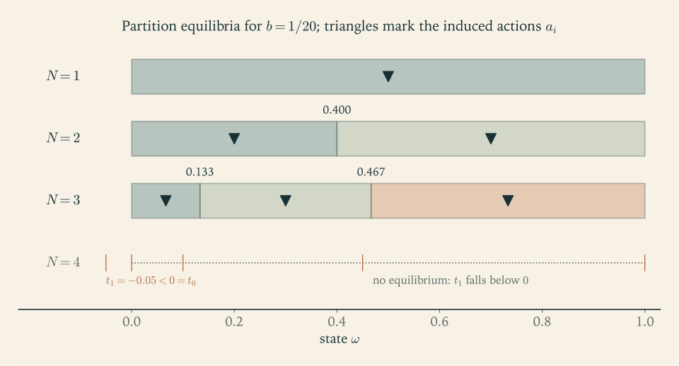
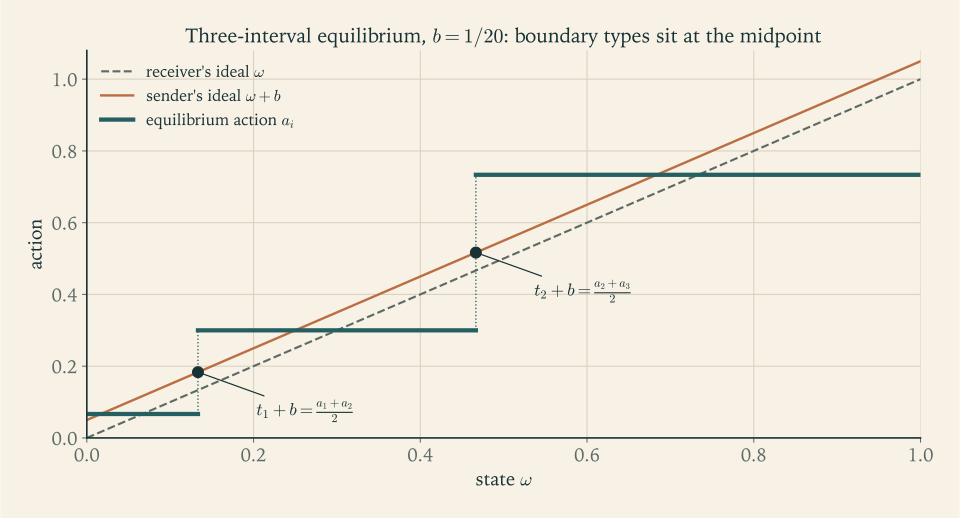
Figure 3.2 shows why the intervals must lengthen. The sender’s ideal line runs a distance \(b\) above the receiver’s. At each boundary, the sender’s ideal must sit at the midpoint of the two steps, and the steps are midpoints of their intervals, which sit on the receiver’s line on average. Because the sender’s line is above the receiver’s, the step above each boundary must reach further up than the step below reaches down, and so the next interval must be longer. The receiver discounts claims of high states, and the coarseness at the top is the form that discount takes in equilibrium.

3.5 Why every equilibrium is an interval equilibrium

The construction of Section 3.4 found the interval equilibria, but it began by assuming the sender uses intervals. Part (a) of Theorem 3.3 says that this was no restriction. The key step is a lemma that limits how close two induced actions can be.

The proof used two features of the model: the receiver’s response is a weighted average of the states that send a message, and every state’s sender wants an action above that state’s receiver-optimal action by a margin bounded away from zero. Crawford and Sobel (1982) prove the same conclusions for a general prior with a positive density, for payoffs that are smooth and strictly concave in the action, for preferences in which higher states want higher actions, and for a sender’s ideal action that always differs from the receiver’s: every equilibrium is outcome-equivalent to a partition equilibrium with finitely many intervals, and the number of intervals is bounded. Under an additional regularity condition, which the uniform–quadratic model satisfies, they also argue that for each feasible \(N\) there is essentially one equilibrium and that equilibria with more intervals are better for both players. Among their results is that an equilibrium with \(N\) intervals implies the existence of one with every smaller number. The theorem is correct, but Kono and Kandori (2021) showed that one assertion in the original proof can fail when the sender’s ideal lies below the receiver’s, and gave a corrected proof. In the uniform–quadratic model, part (c) of Theorem 3.3 establishes existence for every \(N\le N(b)\) directly from the closed form. Exercise 7 works through a nonuniform prior where the midpoint formula fails but the structure survives.

3.6 Counting the cost of the conflict

The partition structure makes welfare a short computation. In an interval of length \(d\) with a uniform posterior, the receiver’s loss is the posterior variance \(d^2/12\) , and the interval has probability \(d\) , so it contributes \(d^3/12\) to the expected loss.

The sender’s loss exceeds the receiver’s by exactly \(b^2\) in every partition equilibrium. The sender, too, suffers from the receiver’s ignorance: her loss consists of the receiver’s error, which she shares, plus the constant disagreement \(b^2\) , which no information can remove. That is why the sender, despite her bias, prefers more informative equilibria. Her interest in exaggerating state by state is at war with her interest, before she knows the state, in a well-informed receiver; Section 3.9 makes this tension precise.

Example 3.4: Welfare across the partitions for a bias of one twentieth

Question. For \(b=1/20\) , compute both players’ expected losses in each of the three equilibria of Example 3.3, and compare with full revelation.

Receiver. By Proposition 3.5 with \(b^2=1/400\) :

\[ L_1=\frac1{12},\qquad L_2=\frac1{48}+\frac{3}{3\cdot400}=\frac{7}{300},\qquad L_3=\frac1{108}+\frac{8}{3\cdot400}=\frac{43}{2700}. \]

As a check on \(L_3\) , sum \(d_i^3/12\) over the intervals of lengths \(\tfrac2{15},\tfrac5{15},\tfrac8{15}\) : \((8+125+512)/(3375\cdot12)=645/40500=43/2700\) .

Sender. Adding \(b^2=1/400\) gives \(103/1200\) , \(31/1200\) , and \(199/10800\) .

Comparison.

Equilibrium	Receiver’s loss	Sender’s loss
Babbling, \(N=1\)	\(1/12\approx0.0833\)	\(103/1200\approx0.0858\)
\(N=2\)	\(7/300\approx0.0233\)	\(31/1200\approx0.0258\)
\(N=3\)	\(43/2700\approx0.0159\)	\(199/10800\approx0.0184\)
Full revelation (not an equilibrium)	\(0\)	\(1/400=0.0025\)

The most informative equilibrium removes about \(81\) percent of the receiver’s babbling loss, since \(1-(43/2700)/(1/12)=1-0.191\) . What remains is more than six times the sender’s own irreducible loss of \(1/400\) . If the sender could somehow be held to full revelation, she would gain \(43/2700\approx0.016\) ; Section 3.9 shows that commitment would do exactly that.

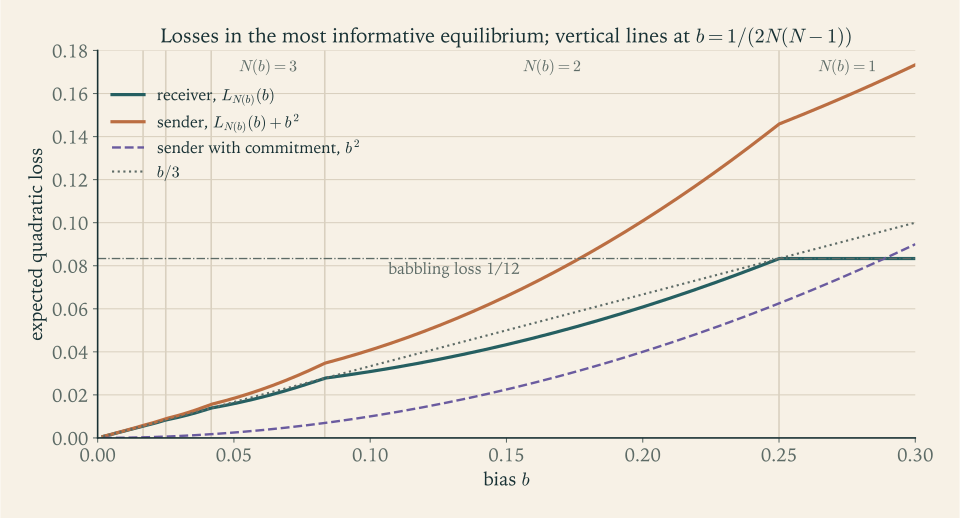
Figure 3.3 shows three things that are not obvious from the formula. The loss is continuous in \(b\) even though \(N(b)\) jumps: at \(b=1/(2N(N-1))\) the first interval of the \(N\) -interval equilibrium shrinks to nothing, and that equilibrium becomes the \((N-1)\) -interval one. The loss never exceeds \(b/3\) and equals it exactly at the jump points (Exercise 11), so for small biases the receiver loses about a third of the bias. And the sender’s loss under cheap talk is far above the \(b^2\) she would bear with commitment, by an amount of order \(b\) rather than \(b^2\) .

A first application of these numbers concerns authority. A receiver who lets the sender choose the action herself suffers loss exactly \(b^2\) , because the sender then picks \(\omega+b\) . Comparing with \(L_{N(b)}(b)\) shows that the receiver should delegate whenever \(b<1/\sqrt{12}\) (Exercise 17), which is Dessein’s (2002) comparison of delegation and communication in organizations.

3.7 Inflated forecasts in a supply chain

Forecast sharing between a buyer and a supplier is a standard operations instance of cheap talk. A manufacturer who will buy a component knows more about its own demand than the supplier who must build capacity, and the manufacturer, which does not pay for the capacity, would like more of it than demand warrants. Cachon and Lariviere (2001) study the contracts that make a forecast credible; the example computes what happens without any contract.

3.8 When the sender’s preferences ignore the state

In Example 3.1 the opposed sender wanted action \(1\) in both states, and no information passed. The general version of that observation concerns senders whose payoff does not depend on the state at all, a situation called transparent motives: a salesperson paid per sale, a lobbyist who wants a bill passed whatever its merits.

The first statement leaves room for informative talk when the sender is indifferent among the actions it induces. If a receiver would take one of two actions the sender likes equally, and an intermediate action she dislikes, then information that moves the receiver away from the intermediate action helps her, and she may reveal it willingly (Exercise 14). Chakraborty and Harbaugh (2010) show that with several dimensions of the state, a sender with transparent motives can often credibly trade off one dimension against another. How much a sender with transparent motives can gain from talk in general is a question with a geometric answer, given at the end of the chapter.

3.9 What commitment would add

Suppose that before learning the state, the sender in the uniform–quadratic model could commit to an experiment, with the receiver seeing the realization and then choosing the action. With a continuum of states, an experiment here means a measurable space \(S\) of realizations together with a Markov kernel \(\pi(\cdot\mid\omega)\in\Delta(S)\) from states to realizations, the posterior after \(s\) being a regular conditional distribution of \(\omega\) given \(s\) . This extends Definition 1.1, which has finitely many states and realizations, and Chapter 8 develops it fully. Full disclosure is the experiment with \(S=[0,1]\) and \(\pi(\cdot\mid\omega)\) the point mass at \(\omega\) . A committed sender does not have to satisfy (S). What would she choose?

The proposition is surprising at first. The sender is biased, yet the experiment she would commit to is the one that serves the receiver perfectly. The reason is that with quadratic payoffs the bias is a constant that information cannot touch, so ex ante the sender’s only stake in information is the receiver’s error, which she shares. The trouble in cheap talk is purely one of timing. Before learning the state the sender wants full revelation; after learning it she wants to exaggerate; and without commitment the receiver anticipates the exaggeration. Commitment closes the gap between the sender’s ex ante and interim interests.

In other games commitment does not lead to full disclosure. Return to the opposed sender of Example 3.1, who wants action \(1\) in both states. Without commitment she gets nothing. With commitment she can choose an experiment that sends the receiver’s posterior either to \(0\) or to \(1/2\) ; by the splitting lemma (Theorem 1.4) the posterior \(1/2\) can have probability \(4/5\) , because \(\tfrac45\cdot\tfrac12=\tfrac25\) is the prior. With ties at \(1/2\) broken in her favor, she obtains action \(1\) with probability \(4/5\) . Chapter 6 develops this calculation into the concavification theorem. The two cases bracket the general picture: commitment always helps the sender weakly, since cheap talk is one of the experiments she could commit to, but how much it helps, and whether the receiver shares in the gain, depends on the shape of her payoffs over beliefs.

3.10 Beyond partitions

Several lines of research start from the uniform–quadratic model. They are signposts here, not developed.

Delegation. Instead of listening, the receiver may hand over the decision, possibly restricting the actions the sender may choose. Holmström (1984) posed the problem of choosing the best set of actions to delegate; Melumad and Shibano (1991) and Alonso and Matouschek (2008) show that the optimal set often takes the form of a cap on the action. Dessein (2002) compares delegation with communication and finds that delegation wins whenever the bias is small enough. Exercise 19 computes the best cap in the uniform–quadratic model.

Selection. Because babbling always coexists with informative equilibria, a prediction requires a selection argument. Farrell (1993) proposed neologism-proofness, which asks whether a new, unused message with a self-signaling meaning would be believed. Chen, Kartik, and Sobel (2008) proposed a criterion called no incentive to separate, which asks that the lowest state not prefer to be identified, and showed that under a regularity condition of Crawford and Sobel, condition (M), which the uniform–quadratic model satisfies, only the equilibrium with \(N(b)\) intervals passes it. That equilibrium is the one usually reported in applications.

Richer protocols. Communication can be improved by several rounds of talk, as Krishna and Morgan (2004) show, by noise in the channel, and by a mediator who garbles the sender’s report before passing it on. Mediated communication is the subject of Chapter 5.

Costs and verification. If lying carries a cost, as in Kartik (2009), the model moves back toward the costly signaling of Game Theory Chapter 8: in the equilibria he studies, language is inflated, low states separate fully, and high states pool. If messages are verifiable but can be withheld, the logic changes entirely, and silence itself becomes informative; that is Chapter 4.

The question this chapter answered was what a biased expert can credibly say when she cannot commit and her words cost nothing. The answer, a finite partition whose coarseness grows with the bias, sets the benchmark against which every other model in the course is measured: Chapter 4 adds verifiable evidence, Chapter 5 a mediator, and Chapter 6 full commitment. Each of those chapters asks which of the three assumptions of Definition 3.1 has been relaxed, and how much of the loss in Figure 3.3 that recovers. One comparison is left open on purpose. For a sender whose preferences ignore the state, Section 3.8 showed that cheap talk can still help her, and Lipnowski and Ravid (2020) measure how much: her best cheap-talk payoff is given by the quasiconcave envelope of her value over beliefs, whereas Chapter 6 will show that her best payoff under commitment is given by the concave envelope. Chapter 10 sets the two envelopes side by side, and Exercise 14 below is the first instance of the question it answers.

Exercises

1. State Definition 3.1 and the three equilibrium conditions (S), (R), (B), and say precisely which feature of the signaling game of Game Theory Definition 8.3 is removed to obtain a cheap-talk game.

   Answer

   A cheap-talk game is a signaling game in the sense of Game Theory Definition 8.3 in which neither payoff depends on the message: \(u_S(\theta,m,a)\) and \(u_R(\theta,m,a)\) are replaced by \(v(a,\omega)\) and \(u(a,\omega)\) . That is the only feature removed. Definition 8.3 already lets every type send every message, so unverifiability is not new; what is new is that sending one message rather than another costs nothing. The conditions are (S) every message sent in state \(\omega\) maximizes \(v(\alpha(m'),\omega)\) over \(m'\) ; (R) \(\alpha(m)\in A^\star(\mu(\cdot\mid m))\) after every message; (B) Bayes’ rule after every message sent with positive probability.

2. For \(b=1/12\) , compute \(N(b)\) , the boundaries and induced actions of every partition equilibrium, and both players’ losses, and explain what goes wrong when the formula of Theorem 3.3 is used to build a three-interval equilibrium at this bias.

   Solution

   The number of intervals. With \(b=1/12\) we have \(1+2/b=25\) , so \(-\tfrac12+\tfrac12\sqrt{25}=2\) and \(N(b)=\lceil 2\rceil=2\) . Directly, \(2bN(N-1)=N(N-1)/6\) equals \(1/3\) at \(N=2\) and exactly \(1\) at \(N=3\) , and the inequality \(2bN(N-1)<1\) is strict.

   One interval. Babbling, with action \(1/2\) . The receiver’s loss is \(1/12\) and the sender’s is \(1/12+1/144=13/144\) .

   Two intervals. Theorem 3.3 gives \(t_1=\tfrac12+2\cdot\tfrac1{12}\cdot1\cdot(1-2)=\tfrac12-\tfrac16=\tfrac13\) . The induced actions are the midpoints \(1/6\) and \(2/3\) . Check the boundary: \(t_1+b=\tfrac13+\tfrac1{12}=\tfrac5{12}\) , and \((\tfrac16+\tfrac23)/2=\tfrac5{12}\) . By Proposition 3.5 the receiver’s loss is

   \[ L_2\!\left(\tfrac1{12}\right)=\frac1{48}+\frac{1}{144}\cdot\frac{3}{3}=\frac1{48}+\frac1{144}=\frac1{36}, \]

   and the sender’s is \(1/36+1/144=5/144\) .

   Three intervals. The formula gives \(t_1=\tfrac13+2\cdot\tfrac1{12}\cdot1\cdot(1-3)=0\) and \(t_2=\tfrac23+2\cdot\tfrac1{12}\cdot2\cdot(2-3)=\tfrac13\) , so the “boundaries” are \(0,0,\tfrac13,1\) . The first interval has length zero. One can still let the single state \(\omega=0\) send a message of its own and receive the action \(0\) : that state’s ideal \(1/12\) is exactly midway between \(0\) and \(1/6\) , so it is indifferent, and the profile satisfies (S), (R), and (B). But the action \(0\) is taken with probability zero, so it is not induced (Section 3.1), and the outcome is that of the two-interval equilibrium. Such a coexisting null action is possible only at threshold biases \(b=1/(2N(N-1))\) , where the first interval of the \(N\) -interval family has length exactly zero. This is the borderline case \(2bN(N-1)=1\) : at \(b=1/12\) the three-interval family has just collapsed into the two-interval one. Consistently, Proposition 3.5 gives \(L_3(1/12)=\tfrac1{108}+\tfrac1{144}\cdot\tfrac83=\tfrac1{36}=L_2(1/12)\) , which is the continuity of the loss visible in Figure 3.3.

3. For \(b=1/100\) , find \(N(b)\) , the first boundary and all interval lengths of the most informative equilibrium, and the receiver’s expected loss, and compare that loss with \(b/3\) .

   Solution

   The number of intervals. With \(b=1/100\) , \(2bN(N-1)=N(N-1)/50\) . This is \(42/50<1\) at \(N=7\) and \(56/50>1\) at \(N=8\) , so \(N(b)=7\) . The formula agrees: \(\sqrt{1+200}=14.18\) , so \(-\tfrac12+\tfrac12\sqrt{201}=6.59\) and the ceiling is \(7\) .

   The partition. The first boundary is

   \[ t_1=\frac17-2\cdot\frac1{100}\cdot 6=\frac17-\frac{3}{25}=\frac{25-21}{175}=\frac{4}{175}. \]

   Each interval is longer than the previous by \(4b=\tfrac{1}{25}=\tfrac{7}{175}\) , so the seven lengths are \(\tfrac{4}{175},\tfrac{11}{175},\tfrac{18}{175},\tfrac{25}{175},\tfrac{32}{175},\tfrac{39}{175},\tfrac{46}{175}\) . They add to \(175/175=1\) , as they must. The boundaries are \(0,\tfrac{4}{175},\tfrac{3}{35},\tfrac{33}{175},\tfrac{58}{175},\tfrac{18}{35},\tfrac{129}{175},1\) .

   The loss. By Proposition 3.5,

   \[ L_7\!\left(\tfrac1{100}\right)=\frac{1}{12\cdot49}+\frac{1}{10000}\cdot\frac{48}{3}=\frac1{588}+\frac{2}{1250}=\frac{1213}{367500}\approx0.003301 . \]

   Comparison. \(b/3=1/300\approx0.003333\) , so the loss is just below \(b/3\) , by about one percent. Exercise 11 shows that this is no accident: the loss in the most informative equilibrium never exceeds \(b/3\) , and for small \(b\) the two are close. Babbling would cost the receiver \(1/12\approx0.0833\) , so the most informative equilibrium removes about \(96\) percent of that loss, since \(0.003301/0.0833=0.040\) .

4. Extending Definition 1.2 to posteriors that are distributions on \([0,1]\) , write the distribution of posteriors \(\tau\) of the two-interval equilibrium for \(b=1/10\) , derive the distribution of the posterior mean, and verify Bayes plausibility (Proposition 1.3) for the mean.

   Answer

   For \(b=1/10\) , \(t_1=3/10\) . The distribution of posteriors puts weight \(3/10\) on the uniform distribution on \([0,\tfrac3{10}]\) and weight \(7/10\) on the uniform distribution on \([\tfrac3{10},1]\) . The posterior mean is \(3/20\) with probability \(3/10\) and \(13/20\) with probability \(7/10\) , and \(\tfrac3{10}\cdot\tfrac3{20}+\tfrac7{10}\cdot\tfrac{13}{20}=\tfrac{9+91}{200}=\tfrac12\) , the prior mean. The weighted average of the two uniform posteriors is the uniform prior, which is Bayes plausibility for the distributions themselves.

5. A student argues: “The sender can always reveal the truth by saying it; in state \(\omega\) she announces \(\omega\) , and since lying costs nothing and gains nothing, truth-telling is an equilibrium.” Find every error in this argument for the uniform–quadratic model with \(b>0\) .

   Solution

   The argument has three errors.

   Messages have no built-in meaning. “Announcing \(\omega\) ” presupposes that a message is understood as a report of the state. In a cheap-talk game a message means whatever the equilibrium makes it mean (Section 3.1); the receiver’s belief after a message is fixed by condition (B) from the sender’s strategy, not by the words.

   Lying does gain something. Suppose the receiver did believe every announcement, responding to “\(r\) ” with \(a=r\) . A sender in state \(\omega\le1-b\) who announces \(\omega+b\) obtains her ideal action \(\omega+b\) and payoff \(0\) , while truth-telling gives \(-(\omega-\omega-b)^2=-b^2<0\) . Condition (S) fails for every such state. The phrase “costs nothing and gains nothing” confuses the cost of the message, which is indeed zero, with its effect on the receiver’s action, which is the whole point of sending it.

   Zero cost is exactly what defeats credibility. In Game Theory Chapter 8 the degree was believed because imitating it was too expensive for the less able type. Here imitation is free, so the only thing that can stop a state from claiming to be a higher state is that the higher state’s action is too far above its own ideal. Lemma 3.4 makes this quantitative: any two induced actions are at least \(2b\) apart, so no equilibrium reveals the state, and the most it can do is report one of at most \(N(b)\) intervals.

   The correct version of the student’s claim is that truth-telling is an equilibrium when \(b=0\) , when the interests coincide.

6. Prove that in no equilibrium of the uniform–quadratic model is the state revealed on an interval of positive length, and show that the receiver rule “respond to the report \(r\) with \(r-b\) ” cannot be part of an equilibrium.

   Hint

   A revealed interval of positive length would carry a continuum of distinct responses to regular messages, one for each state in it; Lemma 3.4 allows at most \(1+1/(2b)\) such responses. For the rule \(r\mapsto r-b\) , ask what report a sender in state \(\omega\) makes when the response to \(r\) is \(r-b\) and her ideal is \(\omega+b\) , and whether the receiver’s rule is then a best response to the reports he actually receives.

7. Let the prior have density \(f(\omega)=2\omega\) on \([0,1]\) , with quadratic payoffs and bias \(b\) ; find the two-interval equilibrium for \(b=1/10\) , and prove that a two-interval equilibrium exists if and only if \(b<1/3\) .

   Solution

   The actions. With density \(f(\omega)=2\omega\) , the conditional mean of the state on an interval \([x,y]\) is

   \[ \frac{\int_x^y 2\omega^2\,d\omega}{\int_x^y 2\omega\,d\omega}=\frac23\cdot\frac{y^3-x^3}{y^2-x^2}=\frac23\cdot\frac{x^2+xy+y^2}{x+y}. \]

   For a two-interval equilibrium with boundary \(t\) , the receiver takes \(a_1=\tfrac23 t\) on \([0,t]\) and \(a_2=\tfrac23\cdot\tfrac{1+t+t^2}{1+t}\) on \([t,1]\) .

   The boundary condition. The sender’s preferences over actions do not involve the prior, so the midpoint rule still says that the state \(t\) must satisfy \(t+b=(a_1+a_2)/2\) , and then states below \(t\) prefer \(a_1\) and states above prefer \(a_2\) . Multiply \(2(t+b)=\tfrac23t+\tfrac23\cdot\tfrac{1+t+t^2}{1+t}\) by \(\tfrac32(1+t)\) :

   \[ 3(t+b)(1+t)=t(1+t)+1+t+t^2\quad\Longleftrightarrow\quad t^2+(1+3b)\,t+3b-1=0 . \]

   For \(b=1/10\) . The equation is \(t^2+1.3\,t-0.7=0\) , whose positive root is

   \[ t=\frac{-13+\sqrt{449}}{20}\approx0.4095 . \]

   The actions are \(a_1\approx0.2730\) and \(a_2\approx0.7460\) , whose midpoint \(0.5095\) equals \(t+b\) . Compared with the uniform prior, where \(t_1=3/10\) , the boundary moves up, because the density puts more weight on high states and the receiver’s actions shift up with it.

   Existence. Let \(h(t)=t^2+(1+3b)t+3b-1\) . A two-interval equilibrium is a root of \(h\) in \((0,1)\) . We have \(h(1)=1+6b>0\) . If \(b<1/3\) then \(h(0)=3b-1<0\) , so by the intermediate value theorem there is a root in \((0,1)\) , and it is unique because the product of the two roots is negative. If \(b\ge1/3\) , the roots have nonnegative product \(3b-1\) and negative sum \(-(1+3b)\) , so neither is positive. Hence a two-interval equilibrium exists exactly when \(b<1/3\) , a weaker requirement than the uniform prior’s \(b<1/4\) .

8. Change the receiver’s payoff to \(-\lvert a-\omega\rvert\) while keeping the uniform prior and the sender’s quadratic payoff; show that the partition equilibria are unchanged, and compute the receiver’s expected loss in the \(N\) -interval equilibrium.

   Hint

   Under the loss \(\lvert a-\omega\rvert\) the receiver’s best response is a median of his posterior. Lemma 3.4’s proof goes through, since every median of a belief lies in the closed convex hull of its support. In the last step of Theorem 3.3(a), replace the tower property of the mean by this fact: a mixture of distributions each having \(a_i\) as a median has \(a_i\) as a median. The conditional distribution of the state given that the receiver takes \(a_i\) is a mixture of the beliefs after the messages leading to \(a_i\) , and it is uniform on \((t_{i-1},t_i)\) , whose only median is the midpoint; so the actions, and every incentive condition of the sender, are those of Section 3.4. The expected loss on an interval of length \(d\) is \(d/4\) , so the receiver’s expected loss is \(\sum_i d_i^2/4=\frac{1}{4N}+\frac{b^2N(N^2-1)}{3}\) , using the interval lengths of Proposition 3.5’s proof; for \(b=1/20\) and \(N=3\) it is \(31/300\) .

9. Prove that in every equilibrium of the uniform–quadratic model, whether or not it was constructed from intervals, the sender’s ex ante expected loss exceeds the receiver’s by exactly \(b^2\) .

   Solution

   Let \((\sigma,\alpha,\mu)\) be any equilibrium and write \(a=\alpha(m)\) for the action taken after the realized message. For the sender,

   \[ E\big[(a-\omega-b)^2\big]=E\big[(a-\omega)^2\big]-2b\,E[a-\omega]+b^2 . \]

   It suffices to show \(E[a-\omega]=0\) . By (R), the response to every message is the mean of the belief after it, and by (B) that belief is a regular conditional distribution of the state given the message, so \(a=E[\omega\mid m]\) almost surely. By the tower property, \(E\big[E[\omega\mid m]\big]=E[\omega]\) , hence \(E[a]=E[\omega]\) and \(E[a-\omega]=0\) . Therefore the sender’s expected loss is the receiver’s plus \(b^2\) . No interval structure was used: the identity relies only on the receiver’s response being the posterior mean, which holds in every equilibrium, partitional or not. The interpretation is that on average the receiver’s action is unbiased, so the sender’s ideal is on average exactly \(b\) away from it, and that systematic gap adds \(b^2\) to whatever error the receiver makes.

10. Derive the formula for \(N(b)\) from the inequality \(2bN(N-1)<1\) , and find the exact set of biases \(b\) for which the most informative equilibrium has three intervals, describing that equilibrium at the smallest such \(b\) .

    Answer

    \(2bN(N-1)<1\) is \(N^2-N-\tfrac1{2b}<0\) , whose positive root is \(\tfrac12+\tfrac12\sqrt{1+2/b}\) ; the largest integer strictly below a real number \(x\) is \(\lceil x\rceil-1=\lceil x-1\rceil\) , which gives the formula. \(N(b)=3\) exactly when \(2b\cdot6<1\le2b\cdot12\) , that is, \(1/24\le b<1/12\) . At \(b=1/24\) the boundaries are \(0,\tfrac16,\tfrac12,1\) and the induced actions are \(\tfrac1{12},\tfrac13,\tfrac34\) .

11. For an integer \(N\ge2\) , show that \(L_N(b)-b/3\) is negative exactly when \(b\) lies strictly between \(1/(2N(N+1))\) and \(1/(2N(N-1))\) , deduce that \(L_{N(b)}(b)\le b/3\) for every \(b>0\) , and find all \(b\) at which equality holds.

    Solution

    The quadratic in \(b\) . By Proposition 3.5,

    \[ L_N(b)-\frac b3=\frac{N^2-1}{3}\,b^2-\frac13\,b+\frac{1}{12N^2}. \]

    Multiplying by \(12N^2>0\) gives \(q(b)=4N^2(N^2-1)b^2-4N^2b+1\) . For \(N\ge2\) the leading coefficient is positive and the discriminant is \(16N^4-16N^2(N^2-1)=16N^2\) , so the roots are

    \[ b=\frac{4N^2\pm4N}{8N^2(N^2-1)}=\frac{N\pm1}{2N(N-1)(N+1)},\quad\text{that is,}\quad b=\frac{1}{2N(N-1)}\ \text{ and }\ b=\frac{1}{2N(N+1)} . \]

    So \(L_N(b)-b/3\) is negative strictly between these roots, zero at them, and positive outside.

    The most informative equilibrium. For \(N\ge2\) , \(N(b)=N\) exactly when \(2bN(N-1)<1\le2bN(N+1)\) , that is, when \(\tfrac{1}{2N(N+1)}\le b<\tfrac{1}{2N(N-1)}\) . On that range \(L_N(b)\le b/3\) , with equality only at the left endpoint. For \(N(b)=1\) , that is \(b\ge1/4\) , the loss is \(1/12\le b/3\) , with equality only at \(b=1/4\) .

    Conclusion. \(L_{N(b)}(b)\le b/3\) for every \(b>0\) , with equality exactly at \(b=1/(2N(N-1))\) for an integer \(N\ge2\) , the biases \(1/4,1/12,1/24,1/40,\dots\) at which \(N(b)\) changes. Each such point is the left end of the range where \(N(b)=N-1\) and the excluded right end of the range where \(N(b)=N\) , which is why the curve in Figure 3.3 touches the line \(b/3\) exactly at the vertical lines.

12. In the three-state game of Example 3.2, find, for every bias \(b>0\) , which of the pure-strategy groupings of the states are equilibria, and identify the most informative equilibrium as a function of \(b\) .

    Answer

    Full revelation is an equilibrium if and only if \(b\le1/2\) ; revealing \(0\) and pooling \(\{1,2\}\) if and only if \(b\le3/4\) ; pooling \(\{0,1\}\) and revealing \(2\) if and only if \(b\le1/4\) ; babbling for every \(b\) . The grouping \(\{0,2\}\) against \(\{1\}\) induces a single action and has the babbling outcome. The most informative equilibrium is full revelation for \(b\le1/2\) , revelation of the low state for \(1/2<b\le3/4\) , and babbling for \(b>3/4\) .

13. In the opposed-interest game of Example 3.1, prove that no equilibrium, even with a mixed sender strategy, induces action \(1\) with positive probability, and compare with what a sender who could commit to an experiment obtains.

    Solution

    No action \(1\) in equilibrium. Allow the sender to mix and the receiver to mix at the indifferent belief \(1/2\) ; write \(r(m)\) for the probability that the receiver takes action \(1\) after \(m\) . The sender’s payoff from sending \(m\) is \(r(m)\) in both states. Let \(r^\star\) be the largest value of \(r(m)\) over the messages that are sent. Any sent message with \(r(m)<r^\star\) is strictly worse, in both states, than a sent message attaining \(r^\star\) , so by (S) it is never sent, a contradiction; hence every sent message has \(r(m)=r^\star\) . Suppose \(r^\star>0\) . The receiver takes action \(1\) with positive probability only at beliefs \(\mu\ge1/2\) , so every posterior after a sent message is at least \(1/2\) . By Proposition 1.3 these posteriors average to the prior \(2/5<1/2\) , a contradiction. So \(r^\star=0\) : in every equilibrium action \(1\) is induced with probability zero, and the sender’s payoff is \(0\) .

    With commitment. A sender who commits to an experiment before the state is drawn can split the prior \(2/5\) into the posteriors \(0\) and \(1/2\) . Bayes plausibility requires \(\tau(\tfrac12)\cdot\tfrac12=\tfrac25\) , so \(\tau(\tfrac12)=4/5\) , and the splitting lemma (Theorem 1.4) supplies an experiment that induces it. With ties broken in her favor, the receiver takes action \(1\) whenever the posterior is \(1/2\) , so the sender obtains action \(1\) with probability \(4/5\) . Commitment raises her payoff from \(0\) to \(4/5\) ; Chapter 6 shows that no experiment does better.

14. With \(\Omega=\{0,1\}\) , prior \(1/2\) , actions \(L\) , \(M\) , \(R\) , receiver payoffs \(u(L,\omega)=1-\omega\) , \(u(R,\omega)=\omega\) , \(u(M,\omega)=3/5\) , and sender payoffs \(\bar v(L)=\bar v(R)=1\) , \(\bar v(M)=0\) , find an informative equilibrium and reconcile it with Proposition 3.6.

    Hint

    At the prior \(1/2\) the actions \(L\) and \(R\) each yield \(1/2<3/5\) , so babbling gives \(M\) and the sender \(0\) . Try truthful reporting: posteriors \(0\) and \(1\) lead to \(L\) and \(R\) , both worth \(1\) to the sender, so she is indifferent and truth-telling satisfies (S). Proposition 3.6 only says that induced actions tie in the sender’s payoff; here \(L\) and \(R\) tie at \(1\) , so it rules nothing out, and its one-to-one clause does not apply because \(\bar v(L)=\bar v(R)\) . Compare her best cheap-talk payoff, \(1\) , with the value of her payoff function at the prior, \(0\) .

15. Let the sender’s payoff be \(-(a-(1-\omega))^2\) in the uniform model with a quadratic receiver, so she wants a high action in low states; prove that every equilibrium has a single induced action.

    Solution

    Work with pure measurable sender strategies as in Section 3.4. Let \(m\) and \(m'\) be regular messages with responses \(a<a'\) . The sender in state \(\omega\) wants the action \(1-\omega\) and, among two actions, prefers the one nearer to it: she weakly prefers \(a\) to \(a'\) exactly when \(1-\omega\le(a+a')/2\) , that is, when \(\omega\ge\hat\omega:=1-(a+a')/2\) . By (S), every state that sends \(m\) weakly prefers \(a\) , since \(m'\) is available, so \(\sigma^{-1}(m)\subseteq[\hat\omega,1]\) ; likewise \(\sigma^{-1}(m')\subseteq[0,\hat\omega]\) . The belief after the regular message \(m\) is concentrated on \(\sigma^{-1}(m)\) , so its mean satisfies \(a\ge\hat\omega\) ; likewise \(a'\le\hat\omega\) . Hence \(a'\le\hat\omega\le a\) , contradicting \(a<a'\) . So all regular messages have the same response, and since regular messages have probability one, the receiver takes a single action \(a^\star\) with probability one. That action is \(E[\omega\mid m]\) almost surely, so by the tower property \(a^\star=E\big[E[\omega\mid m]\big]=E[\omega]=1/2\) , and the outcome is babbling. The contrast with Theorem 3.3 is instructive: there, states that want higher actions are higher states, so a high message points to high states; here they are lower states, and any message that attracted a higher action would be sent by exactly the states for which the receiver wants a lower one.

16. Apply the intuitive criterion of Game Theory Definition 8.4 to the babbling equilibrium of Example 3.1 with aligned interests in which both states send \(m_0\) , and explain why it fails to eliminate this equilibrium.

    Hint

    Take an unsent message \(m_1\) . Under the prior belief the receiver’s best response is action \(0\) , which gives each state of the sender exactly her equilibrium payoff, so \(m_1\) is not equilibrium dominated for either state, and every belief remains admissible. Then ask whether some state gains from \(m_1\) against every admissible best response, including action \(0\) .

17. A firm will choose the scale \(a\) of a new plant, where the right scale \(\omega\) is uniform on \([0,1]\) and known to a consultant who prefers larger projects by \(b=1/8\) ; compare the firm’s loss from listening with its loss from delegating, and find every \(b\) for which delegation is better.

    Solution

    Listening. With \(b=1/8\) , \(2bN(N-1)=N(N-1)/4\) is \(1/2\) at \(N=2\) and \(3/2\) at \(N=3\) , so \(N(1/8)=2\) . The boundary is \(t_1=\tfrac12-2\cdot\tfrac18=\tfrac14\) , the consultant reports whether the right scale is below or above \(1/4\) , and the firm builds \(1/8\) or \(5/8\) . By Proposition 3.5 the firm’s expected loss is

    \[ L_2\!\left(\tfrac18\right)=\frac1{48}+\frac1{64}=\frac{7}{192}\approx0.0365 . \]

    Delegating. If the consultant chooses the scale, she picks her ideal \(\omega+\tfrac18\) , and the firm’s loss is \(b^2=1/64=3/192\approx0.0156\) . Delegation is better, by a factor of more than two.

    For which biases. Delegation gives \(b^2\) and listening gives \(L_{N(b)}(b)\) . If \(N(b)\ge2\) , then \(L_{N(b)}(b)>\tfrac{b^2(N^2-1)}{3}\ge b^2\) because \(N^2-1\ge3\) , so delegation is strictly better. If \(N(b)=1\) , that is \(b\ge1/4\) , listening is babbling with loss \(1/12\) , and delegation is better exactly when \(b^2<1/12\) . Together, delegation is strictly better if and only if \(b<1/\sqrt{12}\approx0.289\) . The firm loses control of the decision, but it gains the use of all of the consultant’s information, and with a small bias that trade is favorable. This is the comparison in Dessein (2002).

18. In Example 3.5, compute the manufacturer’s and the supplier’s expected losses under the cheap-talk equilibrium, under a committed full-disclosure forecast, and under a committed uninformative forecast, and rank the three arrangements for each party.

    Answer

    Manufacturer (sender): cheap talk \(37/1200+1/100=49/1200\approx0.0408\) ; committed full disclosure \(1/100=12/1200\) ; committed uninformative forecast \(1/12+1/100=112/1200\) . Supplier (receiver): \(37/1200\) , \(0\) , and \(1/12=100/1200\) . Both rank full disclosure first, cheap talk second, and no information last, as Proposition 3.7 predicts.

19. The receiver may delegate with a cap, letting the sender choose any action up to \(c\) ; for \(b\le1/2\) , find the cap that minimizes the receiver’s expected loss and show that the minimum loss is \(b^2-4b^3/3\) .

    Solution

    The sender’s choice. Under a cap \(c\) , the sender in state \(\omega\) chooses the allowed action nearest her ideal \(\omega+b\) : she chooses \(\omega+b\) if \(\omega\le c-b\) and \(c\) otherwise.

    The receiver’s loss. For \(b\le c\le1+b\) , states below \(c-b\) cost the receiver \(b^2\) each, and states above cost \((c-\omega)^2\) . With the substitution \(x=c-\omega\) ,

    \[ \Lambda(c)=b^2(c-b)+\int_{c-b}^{1}(c-\omega)^2\,d\omega=b^2(c-b)+\frac{b^3-(c-1)^3}{3}. \]

    The optimal cap. \(\Lambda'(c)=b^2-(c-1)^2\) . On \([b,1-b]\) we have \(1-c\ge b\) , so \(\Lambda'(c)\le0\) ; on \([1-b,1+b]\) we have \(\lvert c-1\rvert\le b\) , so \(\Lambda'(c)\ge0\) . Hence \(\Lambda\) decreases up to \(c=1-b\) and increases after it, and \(c=1-b\) is the minimizer on \([b,1+b]\) ; this interval contains \(1-b\) because \(b\le1/2\) . The minimum is

    \[ \Lambda(1-b)=b^2(1-2b)+\frac{b^3+b^3}{3}=b^2-\frac{4b^3}{3}. \]

    Other caps. A cap \(c\ge1+b\) never binds, giving \(\Lambda=b^2\) , which is larger. A cap \(c<b\) binds for every state, so every state takes \(c\) , and the loss is at least the babbling loss \(1/12\) ; since \(b^2-\tfrac43b^3\) is increasing on \([0,\tfrac12]\) and equals \(1/12\) at \(b=1/2\) , this is no better. The cap at \(1-b\) removes the action from the states near the top, where the sender’s exaggeration is most costly, and lets everyone else choose freely. For \(b=1/8\) the loss falls from \(3/192\) under unrestricted delegation to \(5/384\) .

20. Explain to a procurement manager, in one paragraph without formulas, why a forecast from a buyer with a known incentive to inflate is informative but coarse, and why it is coarser for large orders than for small ones.

    Hint

    Build the paragraph on three points: the buyer gains from overstating, so a precise high forecast would not be believed; a forecast can still separate a low range from a high one, because a buyer with truly low demand does not want the very large capacity that a “high” report would trigger; and each range must be wider than the one below it, because the buyer’s temptation to move up into the next range has to be offset by that range’s capacity being farther above what she wants.

21. (Harder.) In the mixed-strategy setting of the Remark in Section 3.4, prove that almost every message is regular, by showing that the set of state–message pairs in which the message is optimal for the state is measurable and has probability one under the joint law.

    Hint

    Let \(s(\omega)=\sup_{m'}v(\alpha(m'),\omega)\) . Because \(v(a,\omega)=-(a-\omega-b)^2\) , this is \(-d(\omega)^2\) , where \(d(\omega)\) is the distance from \(\omega+b\) to the closure of the set of responses \(\alpha(M)\) ; a distance to a fixed set is continuous, so \(s\) is continuous. The set \(G=\{(\omega,m):v(\alpha(m),\omega)\ge s(\omega)\}\) is then measurable when \(\alpha\) is. Condition (S) says that the section of \(G\) at each \(\omega\) has probability one under \(\sigma(\cdot\mid\omega)\) , so \(G\) has probability one under the joint law. Now disintegrate the joint law along the message: the probability of \(G\) is the average over messages of the belief of its section at \(m\) , which is the set of states for which \(m\) is optimal. An average of numbers at most one equals one only if almost every term equals one.

22. Some texts put the bias on the receiver, with receiver payoff \(-(a-\omega-c)^2\) and sender payoff \(-(a-\omega)^2\) for \(c>0\) ; show that this model’s equilibria come from Theorem 3.3 by shifting actions and reflecting states, and compute the partition for \(c=1/20\) .

    Answer

    Shift actions by \(a'=a-c\) : the receiver’s payoff becomes \(-(a'-\omega)^2\) and the sender’s \(-(a'-\omega+c)^2\) , a downward bias of \(c\) . Reflect states and actions, \(\omega\mapsto1-\omega\) and \(a'\mapsto1-a'\) , which preserves the uniform prior and turns the downward bias into an upward bias \(c\) . So the partitions are those of Theorem 3.3 with \(b=c\) , reflected, and the intervals now shorten as the state rises. For \(c=1/20\) the boundaries are \(0,\tfrac{8}{15},\tfrac{13}{15},1\) , and the receiver’s actions are the interval means plus \(c\) : \(\tfrac{19}{60}\) , \(\tfrac34\) , \(\tfrac{59}{60}\) . At \(\omega=8/15\) the sender’s ideal \(\tfrac{32}{60}\) is the midpoint of \(\tfrac{19}{60}\) and \(\tfrac{45}{60}\) , as indifference requires.