A school cannot make its students more able than they are. It can only decide how to grade them. Suppose two in five of this year’s graduates are able, in the sense that matters to employers, and that employers know this proportion but cannot tell an able graduate from the others by looking at her. Before anyone sits an examination, the school fixes a grading policy: which grades exist, and with what probability a student of each kind receives each grade. An employer who reads a transcript forms a belief about the graduate in front of her. Different policies produce different patterns of belief across the graduating class. A policy that reveals ability exactly leaves two graduates in five known to be able and the rest known not to be. A policy that gives everyone the same grade leaves every graduate at two in five. Between these extremes lie infinitely many others.
Which patterns of belief can a grading policy produce, and which are out of reach? Could the school, for instance, arrange that seven graduates in ten each look at least 60 percent likely to be able? That sounds like a question about the ingenuity of the grading scheme. It is not. Section 1.6 shows by a one-line argument that no scheme whatever can do it, and the bulk of the chapter shows that a single constraint on beliefs is the only one there is: the beliefs a policy produces, weighted by how often they occur, must average to the prior. Every pattern of beliefs that passes this test is produced by some grading policy, and the chapter constructs the policy explicitly.
That result changes what a designer of information is choosing. A grading policy, a credit rating scale, a bank stress test, a platform’s alerts to its drivers: each is a random rule for turning a state of the world into a signal. What matters to anyone who reads the signal is the belief it produces, so the designer may as well choose the beliefs directly, subject to the averaging constraint. Beliefs become the object of choice. The value of information in Chapter 2, persuasion with commitment in Chapters 6 to 8, and information design in games in Chapter 9 are all built on this change of variables, and the chapters on communication without commitment use it to describe what their equilibria reveal.
1.1 Who moves before the state is drawn
The Game Theory course treated beliefs as something players form, not something anyone designs. In a Bayesian game (Game Theory, Definitions 7.1 and 7.2; math.game-theory.bayes-nash-equilibrium) each player’s private information was a type \(\theta_i\)
drawn from a common prior \(p\)
, and a type’s belief about the others was a conditional distribution computed from that prior. In a signaling game (Game Theory, Definition 8.3) the sender first learned her type and then chose a message, and the receiver’s posterior \(\mu(\cdot\mid m)\)
after any message sent with positive probability was pinned down by Bayes’ rule from the sender’s equilibrium strategy: by condition (B) of Game Theory Section 8.3 when the sender uses a pure strategy, and by the consistency condition of Game Theory Definition 8.2 when she mixes, as in the poker game of Game Theory Example 8.4. The posterior was a by-product of equilibrium. Nobody chose it, because each type’s message had to be a best response for that type after she knew it, which is condition (S), and that requirement determined how much the messages revealed.
This course changes the timing and, with it, the vocabulary. The payoff-relevant unknown is now called the state and written \(\omega\) ; it is drawn from a finite set \(\Omega\) with \(n\) elements according to a prior \(\mu_0\in\Delta(\Omega)\) , where \(\Delta(X)\) denotes the set of probability distributions on a set \(X\) . The Game Theory course wrote the private type as \(\theta\) and the prior as \(p\) ; neither symbol is used for these objects again. More importantly, the rule that maps states to signals is chosen before the state is drawn, by someone who is bound by it afterwards. The school chooses its grading policy before the examination; the rating agency publishes its methodology before it rates a borrower; the regulator announces the stress-test scenarios before the banks’ books are opened. Once the rule is fixed, nobody makes any further decision about what to reveal. The state is drawn, the signal is drawn according to the rule, and the reader of the signal updates.
Definition 1.1 (experiment). Let \(\Omega\) be a finite set of states and \(\mu_0\in\Delta(\Omega)\) a prior. An experiment (also called a signal or an information structure) \(\pi=(S,\{\pi(\cdot\mid\omega)\}_{\omega\in\Omega})\) consists of a finite nonempty set \(S\) of signal realizations and, for each state \(\omega\) , a probability distribution \(\pi(\cdot\mid\omega)\in\Delta(S)\) . The state \(\omega\) is drawn from \(\mu_0\) , the realization \(s\) is drawn from \(\pi(\cdot\mid\omega)\) , and an observer who knows \(\mu_0\) and \(\pi\) sees \(s\) but not \(\omega\) . The pair \((\omega,s)\) has probability \(\mu_0(\omega)\pi(s\mid\omega)\) , and the realization \(s\) has probability
A finite experiment is a matrix with one row for each state and one column for each realization, whose rows are probability vectors. The entry in row \(\omega\) and column \(s\) is \(\pi(s\mid\omega)\) , the likelihood of \(s\) in state \(\omega\) . Two experiments mark the ends of the range. Full disclosure \(\bar\pi\) has \(S=\Omega\) and \(\bar\pi(s\mid\omega)=\mathbf 1\{s=\omega\}\) , so its matrix is the identity. No disclosure \(\underline\pi\) has a single realization, so its matrix is a column of ones.
Some papers define an experiment differently: as a joint distribution \(Q\) on \(\Omega\times S\) whose marginal on \(\Omega\) is the prior. The two definitions describe the same objects when the prior has full support. Given a matrix \(\pi\) , the formula \(Q(\omega,s)=\mu_0(\omega)\pi(s\mid\omega)\) defines a joint distribution, and summing over \(s\) returns \(\mu_0(\omega)\) because each row of \(\pi\) sums to one. Conversely, given a joint distribution \(Q\) whose state marginal is \(\mu_0\) , the formula \(\pi(s\mid\omega)=Q(\omega,s)/\mu_0(\omega)\) defines a matrix with nonnegative entries whose rows sum to \(\sum_sQ(\omega,s)/\mu_0(\omega)=1\) . The two formulas undo each other. If some state has prior probability zero, the joint distribution says nothing about that state’s row, which can then be filled in arbitrarily; nothing observable depends on it. The kernel view is the natural one for describing how a test works, and the joint view is the natural one for constructing a test with prescribed results, which is how Section 1.4 will use it.
Nothing in Definition 1.1 says who chose \(\pi\) or why, and that is deliberate. A mixed sender strategy in a signaling game that uses finitely many messages, written \(\sigma(\cdot\mid\omega)\) once the type is renamed the state, is, after the equilibrium is fixed, an experiment in exactly this sense: a map from the state to distributions over messages. Strategies with infinitely many messages, such as the education levels of Game Theory Example 8.3, need the infinite version of the definition that Chapter 8 introduces. So is a grading policy, and so is a medical test with known rates of false positives and false negatives. What differs from one setting to the next is which experiments can arise. In a signaling equilibrium the experiment must respect each type’s incentives after she knows her type. In cheap talk (Chapter 3) it must survive the sender’s temptation to misreport at no cost. With verifiable evidence (Chapter 4) it is limited by what can be proved. Under full commitment (Chapter 6) the designer may pick any experiment at all. This chapter studies what an experiment does to beliefs, whatever its origin, so its results hold in all of those settings at once.
1.2 Reading a grade
An observer who knows \(\pi\)
and sees \(s\)
updates by Bayes’ rule: for events \(E\)
and \(F\)
with \(\Pr(F)>0\)
, \(\Pr(E\mid F)=\Pr(E\cap F)/\Pr(F)\)
, from Probability Theory (math.probability-theory.bayes-rule). Here \(E\)
is the event that the state is \(\omega\)
, and \(F\)
is the event that the realization is \(s\)
.
Definition 1.2 (distribution of posteriors). Let \(\mu_0\) be a prior and \(\pi\) an experiment. For each realization \(s\) with \(\pi(s)>0\) , the posterior after \(s\) is the belief \(\mu_s\in\Delta(\Omega)\) given by
The distribution of posteriors of \(\pi\) is the probability distribution \(\tau_\pi\in\Delta(\Delta(\Omega))\) that gives each belief \(\mu\) the total probability of the realizations leading to it:
Its support \(\operatorname{supp}\tau_\pi\) is the finite set of posteriors that occur with positive probability. When the experiment is clear from the context, the subscript is dropped and the distribution is written \(\tau\) .
Three features of the definition deserve comment. First, \(\tau_\pi\) forgets the names of the realizations. A grade called A and a grade called B that lead to the same posterior become one point of the support, and their probabilities are added. Second, realizations with \(\pi(s)=0\) do not enter. Their posteriors are undefined, and because they are never observed, they never matter. This is a real departure from Game Theory Section 8.3, where the receiver’s belief after a message that no type sends was a free and consequential part of the equilibrium: it was what deterred deviations. A committed experiment cannot be deviated from, so there is nothing to deter. Third, \(\tau_\pi\) depends on the prior as well as on \(\pi\) . The same grading matrix applied to a weaker cohort produces different beliefs.
When the state is binary, \(\Omega=\{0,1\}\) , a belief is identified with the single number \(\mu=\Pr(\omega=1)\in[0,1]\) , and the prior with \(\mu_0\in(0,1)\) . This convention is in force whenever the state is binary. Bayes’ rule is quickest in odds form: for a realization with \(\pi(s\mid 0)>0\) , the posterior odds \(\mu_s/(1-\mu_s)\) equal the prior odds \(\mu_0/(1-\mu_0)\) times the likelihood ratio \(\pi(s\mid 1)/\pi(s\mid 0)\) .
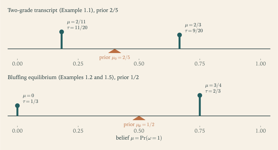
Example 1.1: A two-grade transcript and a three-grade one
Let \(\omega=1\) mean that a graduate is able, with prior \(\mu_0=2/5\) . The school awards a Distinction or a Pass, written \(D\) and \(P\) . It gives \(D\) to an able student with probability \(3/4\) and to any other student with probability \(1/4\) :
Probabilities of the grades. The joint probabilities of an able student with each grade are \(\tfrac25\cdot\tfrac34=\tfrac{6}{20}\) and \(\tfrac25\cdot\tfrac14=\tfrac{2}{20}\) ; for the other students they are \(\tfrac35\cdot\tfrac14=\tfrac{3}{20}\) and \(\tfrac35\cdot\tfrac34=\tfrac{9}{20}\) . Adding down each grade gives \(\pi(D)=\tfrac{9}{20}\) and \(\pi(P)=\tfrac{11}{20}\) .
Posteriors. Dividing each grade’s able entry by the grade’s total,
In odds form, the prior odds are \(2/3\) . A Distinction has likelihood ratio \(3\) , which gives odds \(2\) and posterior \(2/3\) ; a Pass has likelihood ratio \(1/3\) , which gives odds \(2/9\) and posterior \(2/11\) .
Distribution of posteriors. \(\tau(2/3)=9/20\) and \(\tau(2/11)=11/20\) . Its mean is
which is the prior.
A three-grade transcript. Now let the school award A, B, or C with
The likelihood ratios are \(3\) , \(3\) , and \(1/3\) , so grades A and B both lead to the posterior \(2/3\) and grade C leads to \(2/11\) . The grade probabilities are \(\pi(A)=\tfrac15+\tfrac1{10}=\tfrac{3}{10}\) , \(\pi(B)=\tfrac1{10}+\tfrac1{20}=\tfrac{3}{20}\) , and \(\pi(C)=\tfrac1{10}+\tfrac{9}{20}=\tfrac{11}{20}\) . Merging A and B gives \(\tau(2/3)=\tfrac3{10}+\tfrac3{20}=\tfrac9{20}\) and \(\tau(2/11)=\tfrac{11}{20}\) , which is exactly the distribution of posteriors of the two-grade transcript.
The two transcripts look different on paper. One has an extra grade, and a casual reader might think a B means something different from an A. It does not: an employer who knows the policy reaches the same belief after either, and the population of employer beliefs is identical under the two policies. Experiments with the same distribution of posteriors are equivalent for every decision maker, whatever decision she faces. Chapter 2 proves this once decision problems are defined (Definition 2.1), but the reason is already visible. A reader of the transcript can act only on what she believes, and the two policies produce the same beliefs with the same frequencies.
Common mistake. Reading a likelihood as a posterior. A recruiter told that three quarters of able students receive a Distinction concludes that a graduate holding one is able with probability \(3/4\) . That figure is \(\pi(D\mid 1)\) , the probability of the grade given the state. The recruiter needs \(\mu_D\) , the probability of the state given the grade, which Example 1.1 computed to be \(2/3\) . The two differ because the recruiter has ignored the base rate: three graduates in five are not able, a quarter of them also receive a Distinction, and they account for a third of all Distinctions awarded. The repair is to write out the joint probabilities \(\mu_0(\omega)\pi(s\mid\omega)\) before dividing; a posterior is one column of that table, rescaled to sum to one. The likelihood and the posterior coincide only in special cases, such as a symmetric test applied at the prior \(1/2\) .
The same translation turns the equilibria of Game Theory Chapter 8 into distributions of posteriors.
Example 1.2: A bluffing equilibrium as a distribution of posteriors
In the one-card poker game of Game Theory Example 8.4 the sender holds High or Low with probability \(1/2\)
each. In its perfect Bayesian equilibrium (Game Theory, Definition 8.2; math.game-theory.perfect-bayesian-equilibrium) High always bets and Low bets with probability \(1/3\)
. Let \(\omega=1\)
mean High, so \(\mu_0=1/2\)
. The sender’s equilibrium strategy is the experiment with realizations Bet and Fold and likelihoods
Then \(\pi(\mathrm{Bet})=\tfrac12+\tfrac16=\tfrac23\) and \(\pi(\mathrm{Fold})=\tfrac13\) . The posteriors are \(\mu_{\mathrm{Bet}}=\tfrac12\big/\tfrac23=\tfrac34\) , as Game Theory found from the receiver’s indifference, and \(\mu_{\mathrm{Fold}}=0\) , since only Low ever folds. The equilibrium’s distribution of posteriors is
The receiver takes no action after a fold, but the belief is defined, and it is \(0\) .
The three kinds of equilibrium in Game Theory Section 8.3 translate in the same way. A separating equilibrium with two types produces the distribution of posteriors of full disclosure: the posterior \(1\) with the prior probability of the first type and \(0\) with that of the second. A pooling equilibrium produces the point mass at the prior. A partially separating equilibrium, like the poker one, moves the posteriors away from the prior without making them all certain. In the poker game the bluffing frequency \(1/3\) was not chosen to produce any particular pattern of beliefs; it was forced by the receiver’s indifference condition, which fixes the posterior after a bet at \(3/4\) . Section 1.6 shows, with some surprise, that a designer who wanted the receiver to believe High with probability at least \(3/4\) as often as possible would choose exactly this distribution.
Example 1.3: A credit rating with three states
A rating agency classifies a borrower as good, marginal, or bad, written \(G\) , \(M\) , \(B\) , with prior \(\mu_0=(\tfrac12,\tfrac3{10},\tfrac15)\) in the order \((G,M,B)\) . It issues one of three ratings, AA, A, or C, with likelihoods
Joint probabilities. Multiplying each row by its prior probability gives
Rating probabilities. The column sums are \(\pi(\mathrm{AA})=\tfrac{7}{20}\) , \(\pi(\mathrm{A})=\tfrac{8}{20}=\tfrac25\) , and \(\pi(\mathrm{C})=\tfrac{5}{20}=\tfrac14\) .
Posteriors. Rescaling each column to sum to one,
Bayes plausibility. The weighted sum is
Each rating says something different. An AA rules out a bad borrower entirely, since the agency never gives AA to one. An A makes a marginal borrower the most likely of the three. A C still leaves a one-in-five chance that the borrower is good. Figure 1.2 in Section 1.5 places these three posteriors in the triangle of beliefs.
1.3 The one restriction on posteriors
The calculations of the three examples ended with the same check, and it never failed.
Proposition 1.3 (Bayes plausibility). For every prior \(\mu_0\) and every experiment \(\pi\) , the distribution of posteriors averages to the prior:
A finite-support distribution \(\tau\in\Delta(\Delta(\Omega))\) that satisfies \(E_\tau[\mu]=\mu_0\) is called Bayes plausible.
Proof. Fix a state \(\omega\) . If a realization has \(\pi(s)=0\) , every term of the sum \(\sum_{\omega'}\mu_0(\omega')\pi(s\mid\omega')\) is zero, and in particular \(\mu_0(\omega)\pi(s\mid\omega)=0\) . Grouping the realizations by the posterior they produce, and using Definition 1.2 to write \(\pi(s)\mu_s(\omega)=\mu_0(\omega)\pi(s\mid\omega)\) ,
The third equality adds back the zero terms, and the last uses \(\sum_{s}\pi(s\mid\omega)=1\) . Since \(\omega\) was arbitrary, the vectors agree.
The computation is the law of total probability, \(\Pr(\omega)=\sum_s\Pr(s)\Pr(\omega\mid s)\)
, read with the realization as the conditioning variable. It has a more general form that will be needed in Section 1.7. Regard the posterior \(\mu_s\)
as a random vector, a function of the random realization. For each state \(\omega\)
, the number \(\mu_s(\omega)\)
is the conditional expectation of the indicator of the event that the state is \(\omega\)
, given the realization. The tower property says that for an integrable random variable \(X\)
and any random variable \(Y\)
on the same probability space, \(E[E[X\mid Y]]=E[X]\)
(from Probability Theory; math.probability-theory.tower-property). With \(X\)
the indicator and \(Y\)
the realization, it gives \(E[\mu_s(\omega)]=\mu_0(\omega)\)
, which is Proposition 1.3 again. When experiments are run one after another, the same property says that the sequence of beliefs is a martingale: each new belief is, on average, the belief held just before it.
Proposition 1.3 has a blunt reading: no experiment moves the expected belief. A school that wants employers to think better of its graduates on average cannot achieve it by grading, however cleverly, because the average employer belief across the class is the share of able graduates, whatever the transcript says. What grading can do is spread the beliefs out, making some graduates look better and others worse. The question of this chapter is which spreads are possible.
Common mistake. Concluding from Proposition 1.3 that information cannot change what people do on average. The expected belief is fixed; expected behaviour is not, because behaviour need not be linear in beliefs. Take the employer of Game Theory Example 8.2, who strictly prefers the skilled job when the probability of an able applicant exceeds \(3/4\) and is indifferent at exactly \(3/4\) . Break that tie toward the skilled job, and let the prior be \(1/2\) . With no information, every applicant sits at the prior and nobody gets the skilled job. Under the experiment of Example 1.2, two applicants in three sit at the posterior \(3/4\) and get it. The average belief is \(1/2\) in both cases, while the share of skilled assignments rises from \(0\) to \(2/3\) . What Proposition 1.3 fixes is the expectation of the belief and of anything linear in the belief, such as the expected productivity of the applicant pool; a threshold rule is not linear. Chapter 2 builds the value of information on this observation, and Chapter 6 builds the value of persuasion on it.
1.4 Splitting a prior
Proposition 1.3 is a necessary condition on the distributions of posteriors that experiments can produce. The central fact of the chapter is that it is also sufficient.
Theorem 1.4 (splitting lemma). Let the prior \(\mu_0\in\Delta(\Omega)\) have full support, and let \(\tau\in\Delta(\Delta(\Omega))\) have finite support and be Bayes plausible. Define an experiment \(\pi\) whose realization set is \(S=\operatorname{supp}\tau\) by
Then \(\pi\) is an experiment; the realization \(\mu\) occurs with probability \(\pi(\mu)=\tau(\mu)\) ; the posterior after the realization \(\mu\) is \(\mu\) itself; and \(\tau_\pi=\tau\) .
Proof. Step 1: \(\pi\) is an experiment. Each entry is nonnegative, because \(\tau(\mu)\ge 0\) , \(\mu(\omega)\ge 0\) , and \(\mu_0(\omega)>0\) . For each state \(\omega\) , Bayes plausibility gives
so each \(\pi(\cdot\mid\omega)\) is a probability distribution on \(S\) .
Step 2: the probability of each realization. For \(\mu\in S\) ,
Step 3: the posterior after each realization. By Definition 1.2 and Step 2,
Step 4: the distribution of posteriors. The realizations are distinct elements of \(\operatorname{supp}\tau\) , and by Step 3 each produces itself as posterior, so no two realizations share a posterior. Hence \(\tau_\pi(\mu)=\pi(\mu)=\tau(\mu)\) for every \(\mu\in S\) , and \(\tau_\pi\) puts no mass outside \(S\) .
The formula is Bayes’ rule run backwards, and the joint view of an experiment from Section 1.1 shows why it must be this one. We want the posterior \(\mu\) to appear with frequency \(\tau(\mu)\) , so the joint probability of the state \(\omega\) together with the realization \(\mu\) has to be \(\tau(\mu)\mu(\omega)\) : the probability of the realization times the probability of the state given the realization. A joint distribution on states and realizations is an experiment only if its state marginal is the prior, and the state marginal of this one is \(\sum_\mu\tau(\mu)\mu(\omega)\) . Bayes plausibility is precisely the statement that the target joint distribution has the right marginal. Dividing by the prior then turns the joint distribution into the kernel of Definition 1.1.
The result is usually attributed to Aumann and Maschler, whose research reports of 1966 to 1968 for the United States Arms Control and Disarmament Agency, on repeated games with incomplete information and later collected in a book with Stearns (Aumann and Maschler 1995), studied an informed player who reveals information by letting her actions depend on her type. The name describes that setting, where the player’s behaviour splits the prior into a collection of posteriors. Kamenica and Gentzkow (2011) made the same characterization the starting point of Bayesian persuasion.
The full-support hypothesis serves only to make the division in Theorem 1.4 legitimate, and it can be dropped.
Corollary 1.5 (feasible distributions of posteriors). Let \(\mu_0\in\Delta(\Omega)\) be any prior. A finite-support distribution \(\tau\in\Delta(\Delta(\Omega))\) is the distribution of posteriors of some experiment if and only if it is Bayes plausible.
Proof. Necessity is Proposition 1.3. For sufficiency, let \(\Omega_0=\{\omega:\mu_0(\omega)>0\}\) . For \(\omega\notin\Omega_0\) , Bayes plausibility gives \(\sum_\mu\tau(\mu)\mu(\omega)=0\) , a sum of nonnegative terms, so \(\mu(\omega)=0\) for every \(\mu\) in the support of \(\tau\) . Define \(\pi(\mu\mid\omega)\) by the formula of Theorem 1.4 for \(\omega\in\Omega_0\) , and let \(\pi(\cdot\mid\omega)\) be any distribution on \(\operatorname{supp}\tau\) for \(\omega\notin\Omega_0\) . States outside \(\Omega_0\) contribute nothing to any realization probability or posterior, and each \(\mu\) in the support satisfies \(\sum_{\omega\in\Omega_0}\mu(\omega)=1\) . Steps 1 to 4 of the proof of Theorem 1.4 therefore go through with sums over \(\Omega_0\) , and the posterior after \(\mu\) equals \(\mu\) on \(\Omega_0\) and \(0\) off it, which is \(\mu\) .
Corollary 1.5 converts every question of the form “which experiment should be chosen?” into the question “which Bayes-plausible distribution of posteriors should be chosen?”, provided whatever is at stake depends on the realization only through the posterior it produces. The second question is posed in a fixed convex set, the Bayes-plausible distributions, and does not mention signal realizations at all. Chapter 6 solves persuasion problems in exactly this form.
The splitting experiment has a special property: each realization is a belief, and it is the belief that a Bayesian reader holds after seeing it.
Definition 1.6 (direct experiment). An experiment is direct if its realization set \(S\) is a finite subset of \(\Delta(\Omega)\) and each realization \(\mu\in S\) with \(\pi(\mu)>0\) produces the posterior \(\mu\) .
A direct experiment’s realization reads as a message, “your belief should now be \(\mu\)
”, which a reader who does Bayes’ rule finds to be correct. The idea has a close relative in the revelation principle (Game Theory, Theorem 9.4; math.game-theory.revelation-principle). There, any mechanism could be replaced by a direct one in which each bidder reports his value; here, any experiment can be replaced by a direct one in which each realization is labeled by the belief it produces. Chapters 5 and 7 meet a third relabeling, in which realizations are labeled by the action they lead the receiver to take.
Proposition 1.7 (merging realizations). Let \(\mu_0\) have full support and let \(\pi\) be an experiment.
(a) Define \(\pi^{\mathrm d}\) with realization set \(\operatorname{supp}\tau_\pi\) and \(\pi^{\mathrm d}(\mu\mid\omega)=\sum_{s:\ \pi(s)>0,\ \mu_s=\mu}\pi(s\mid\omega)\) . Then \(\pi^{\mathrm d}\) is a direct experiment and \(\tau_{\pi^{\mathrm d}}=\tau_\pi\) .
(b) If a direct experiment \(\pi'\) with realization set \(S'\) has distribution of posteriors \(\tau\) , then \(\pi'(\mu\mid\omega)=\tau(\mu)\mu(\omega)/\mu_0(\omega)\) for every \(\mu\in\operatorname{supp}\tau\) and every \(\omega\) , and \(\pi'(\mu\mid\omega)=0\) for every \(\mu\in S'\) outside \(\operatorname{supp}\tau\) . In particular, the only direct experiment inducing \(\tau\) , up to realizations that never occur, is the splitting experiment of Theorem 1.4, and \(\pi^{\mathrm d}\) is the splitting experiment of \(\tau_\pi\) .
Proof. (a) Because the prior has full support, \(\pi(s)=0\) forces \(\pi(s\mid\omega)=0\) for every \(\omega\) . So \(\sum_\mu\pi^{\mathrm d}(\mu\mid\omega)=\sum_{s:\ \pi(s)>0}\pi(s\mid\omega)=\sum_{s\in S}\pi(s\mid\omega)=1\) . The probability of the realization \(\mu\) is \(\sum_\omega\mu_0(\omega)\sum_{s:\ \mu_s=\mu}\pi(s\mid\omega)=\sum_{s:\ \mu_s=\mu}\pi(s)=\tau_\pi(\mu)>0\) , and its posterior is
where the sums run over realizations of positive probability. So \(\pi^{\mathrm d}\) is direct, its realizations produce distinct posteriors, and \(\tau_{\pi^{\mathrm d}}(\mu)=\tau_\pi(\mu)\) .
(b) Let \(\mu\in S'\) have \(\pi'(\mu)>0\) . Directness says \(\mu(\omega)=\mu_0(\omega)\pi'(\mu\mid\omega)/\pi'(\mu)\) , that is, \(\pi'(\mu\mid\omega)=\pi'(\mu)\mu(\omega)/\mu_0(\omega)\) . Realizations of positive probability produce themselves, so distinct ones produce distinct posteriors, and therefore \(\tau(\mu)=\pi'(\mu)\) . This gives the formula and shows that every realization of positive probability lies in \(\operatorname{supp}\tau\) ; conversely, each point of \(\operatorname{supp}\tau\) is the posterior of some realization of positive probability, which must be that point itself. If \(\mu\in S'\) has \(\pi'(\mu)=0\) , full support of the prior gives \(\pi'(\mu\mid\omega)=0\) for every \(\omega\) . Applying (b) to the direct experiment \(\pi^{\mathrm d}\) of part (a) proves the last claim.
Taken together, Proposition 1.7 and Theorem 1.4 say precisely what is lost in passing from an experiment to its distribution of posteriors: the names of the realizations, and the way a single posterior is divided among several realizations. Nothing a Bayesian reader could ever act on is lost.
Example 1.4: Building a rating to order
Keep the borrowers of Example 1.3, with prior \(\mu_0=(\tfrac12,\tfrac3{10},\tfrac15)\) . An investor group first asks the agency for a rating scale under which no rating leaves investors more than \(40\) percent confident that the borrower is good. No experiment can deliver that. Every posterior would then have \(\mu(G)\le\tfrac25\) , so any average of posteriors would have \(G\) -coordinate at most \(\tfrac25\) , while Proposition 1.3 requires the average to be \(\tfrac12\) .
The group revises its request. It now wants three ratings, prime, standard, and watch, producing the posteriors
A prime borrower is certainly good, a standard borrower is certainly not bad, and a watch borrower is bad with probability one half.
Step 1: the weights. A Bayes-plausible \(\tau\) on these posteriors must satisfy \(\tau_1\mu^1+\tau_2\mu^2+\tau_3\mu^3=\mu_0\) , where \(\tau_j\) abbreviates \(\tau(\mu^j)\) . Reading the coordinates from the last to the first,
The first gives \(\tau_3=\tfrac25\) ; the second gives \(\tfrac34\tau_2=\tfrac3{10}-\tfrac1{10}=\tfrac15\) , so \(\tau_2=\tfrac4{15}\) ; the third gives \(\tau_1=\tfrac12-\tfrac1{15}-\tfrac1{10}=\tfrac13\) . The weights are positive and sum to \(\tfrac13+\tfrac4{15}+\tfrac25=1\) , so \(\tau\) is Bayes plausible and the request can be met.
Step 2: the experiment. Theorem 1.4 sets \(\pi(\mu^j\mid\omega)=\tau_j\mu^j(\omega)/\mu_0(\omega)\) . For a good borrower, \(\pi(\mu^1\mid G)=\tfrac13\cdot 1\big/\tfrac12=\tfrac23\) , \(\pi(\mu^2\mid G)=\tfrac4{15}\cdot\tfrac14\big/\tfrac12=\tfrac2{15}\) , and \(\pi(\mu^3\mid G)=\tfrac25\cdot\tfrac14\big/\tfrac12=\tfrac15\) . Completing the table,
Each row sums to one, as Step 1 of the proof of Theorem 1.4 guarantees.
Step 3: verification. The standard rating has probability \(\tfrac12\cdot\tfrac2{15}+\tfrac3{10}\cdot\tfrac23=\tfrac1{15}+\tfrac15=\tfrac4{15}\) , and its posterior is \(\bigl(\tfrac1{15},\tfrac15,0\bigr)\big/\tfrac4{15}=\bigl(\tfrac14,\tfrac34,0\bigr)\) . The watch rating has probability \(\tfrac12\cdot\tfrac15+\tfrac3{10}\cdot\tfrac13+\tfrac15\cdot 1=\tfrac25\) , and its posterior is \(\bigl(\tfrac1{10},\tfrac1{10},\tfrac15\bigr)\big/\tfrac25=\bigl(\tfrac14,\tfrac14,\tfrac12\bigr)\) . The prime rating has probability \(\tfrac12\cdot\tfrac23=\tfrac13\) and posterior \((1,0,0)\) .
In words: every bad borrower is put on watch; a marginal borrower is rated standard two times in three and watch otherwise; a good borrower is rated prime two times in three, standard with probability \(2/15\) , and watch with probability \(1/5\) . The agency did not need to guess this table. It chose the beliefs, and Theorem 1.4 produced the rule.
1.5 Pictures in the simplex
Bayes plausibility is a statement about centres of mass, and it is easiest to understand in a picture.
With a binary state, beliefs are points of the interval \([0,1]\) . A distribution of posteriors is a finite collection of masses placed on the interval, and Bayes plausibility says that their centre of mass is the prior. With two posteriors \(\mu_L<\mu_0<\mu_H\) this is the law of the lever: the weights are inversely proportional to the distances from the prior,
The farther a posterior lies from the prior, the less often it can occur. In Example 1.1 the Pass posterior \(2/11\) is \(12/55\) below the prior and the Distinction posterior \(2/3\) is \(4/15\) above it; the weights \(11/20\) and \(9/20\) satisfy \(\tfrac{11}{20}\cdot\tfrac{12}{55}=\tfrac{9}{20}\cdot\tfrac{4}{15}=\tfrac{3}{25}\) , which is the lever balancing.
With three states, \(\Delta(\Omega)\) is a triangle in \(\mathbb R^3\) : the set of vectors \((\mu(\omega_1),\mu(\omega_2),\mu(\omega_3))\) with nonnegative entries summing to one. Its vertices are the beliefs certain of one state; its edges are the beliefs that rule out one state; and a belief’s coordinates are its barycentric coordinates with respect to the vertices, so the belief \((\tfrac12,\tfrac3{10},\tfrac15)\) is the point that would balance masses \(\tfrac12\) , \(\tfrac3{10}\) , \(\tfrac15\) placed at the three vertices. A distribution of posteriors places masses at points of the triangle, and Bayes plausibility again says that the prior is their centre of mass. In particular, the prior lies in the convex hull of the support of \(\tau\) . Figure 1.2 draws the posteriors of Examples 1.3 and 1.4.
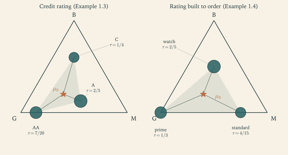
The picture answers two practical questions: which collections of posteriors can support a Bayes-plausible distribution, and how many different weightings there are.
Proposition 1.8 (weights and supports). Let \(\mu_0\in\Delta(\Omega)\) and \(n=\lvert\Omega\rvert\) .
(a) Let \(\mu^1,\dots,\mu^k\in\Delta(\Omega)\) be affinely independent. A Bayes-plausible \(\tau\) supported in \(\{\mu^1,\dots,\mu^k\}\) exists if and only if \(\mu_0\) lies in the convex hull of \(\mu^1,\dots,\mu^k\) . It is then unique, and \(\tau(\mu^j)\) is the \(j\) -th barycentric coordinate of \(\mu_0\) with respect to \(\mu^1,\dots,\mu^k\) . Its support is all of \(\{\mu^1,\dots,\mu^k\}\) exactly when every coordinate is positive.
(b) In the binary case, if \(\mu_L<\mu_0<\mu_H\) , the unique Bayes-plausible distribution on \(\{\mu_L,\mu_H\}\) has \(\tau(\mu_H)=(\mu_0-\mu_L)/(\mu_H-\mu_L)\) and \(\tau(\mu_L)=(\mu_H-\mu_0)/(\mu_H-\mu_L)\) .
(c) Let \(f:\Delta(\Omega)\to\mathbb R\) be any function. For every Bayes-plausible \(\tau\) there is a Bayes-plausible \(\tau'\) with \(\operatorname{supp}\tau'\subseteq\operatorname{supp}\tau\) , at most \(n\) points in its support, and \(E_{\tau'}[f(\mu)]\ge E_\tau[f(\mu)]\) .
Proof. (a) A distribution supported in \(\{\mu^1,\dots,\mu^k\}\) is a vector \(\lambda\in\mathbb R^k\) with \(\lambda_j\ge 0\) and \(\sum_j\lambda_j=1\) , and it is Bayes plausible exactly when \(\sum_j\lambda_j\mu^j=\mu_0\) . Such a vector is a representation of \(\mu_0\) as a convex combination of the \(\mu^j\) , so one exists exactly when \(\mu_0\) is in their convex hull. If \(\lambda\) and \(\lambda'\) are two such vectors, then \(\sum_j(\lambda_j-\lambda'_j)\mu^j=0\) and \(\sum_j(\lambda_j-\lambda'_j)=0\) , and affine independence forces \(\lambda=\lambda'\) . The coefficients of the unique representation are by definition the barycentric coordinates, and the support is the set of \(j\) with \(\lambda_j>0\) .
(b) Two distinct numbers are affinely independent, and \(\mu_0\) lies between them. Solving \(\lambda\mu_H+(1-\lambda)\mu_L=\mu_0\) gives \(\lambda=(\mu_0-\mu_L)/(\mu_H-\mu_L)\) .
(c) Let \(\operatorname{supp}\tau=\{\mu^1,\dots,\mu^k\}\) with weights \(\lambda_j>0\) , and suppose \(k>n\) . The \(k-1\) vectors \(\mu^j-\mu^1\) , for \(j=2,\dots,k\) , lie in the subspace \(\{x\in\mathbb R^\Omega:\sum_\omega x(\omega)=0\}\) , which has dimension \(n-1<k-1\) . They are therefore linearly dependent: there are numbers \(d_2,\dots,d_k\) , not all zero, with \(\sum_{j\ge 2}d_j(\mu^j-\mu^1)=0\) . Put \(c_j=d_j\) for \(j\ge 2\) and \(c_1=-\sum_{j\ge 2}d_j\) ; then \(\sum_jc_j\mu^j=0\) and \(\sum_jc_j=0\) , with the \(c_j\) not all zero. Because the \(c_j\) sum to zero and are not all zero, both \(c\) and \(-c\) have a positive entry, so replacing \(c\) by \(-c\) if necessary we may assume \(\sum_jc_jf(\mu^j)\le 0\) and still have some \(c_j>0\) . Let \(t=\min\{\lambda_j/c_j:c_j>0\}\) and \(\lambda'_j=\lambda_j-tc_j\) . Then every \(\lambda'_j\ge 0\) , \(\sum_j\lambda'_j=1\) , \(\sum_j\lambda'_j\mu^j=\mu_0\) , at least one \(\lambda'_j\) is zero, and
Dropping the points with zero weight leaves a Bayes-plausible distribution with a smaller support inside the old one and an expectation of \(f\) at least as large. Repeating the step while the support has more than \(n\) points proves the claim.
With \(f\) identically zero, part (c) is Carathéodory’s theorem for the simplex. With a general \(f\) it has a consequence that later chapters use repeatedly: a designer who wants to maximize the expectation of a function of the posterior loses nothing by restricting attention to experiments with at most as many realizations as there are states, because every experiment can be replaced by one with at most \(n\) posteriors that does at least as well. The guarantee is one of improvement, not of equality. To reproduce an exact value of \(E_\tau[f(\mu)]\) , apply Carathéodory’s theorem to the points \((\mu,f(\mu))\) , which live in a space of affine dimension \(n\) ; that argument needs up to \(n+1\) posteriors, and with a binary state some values do require three. Part (a) is the reason the weights in Example 1.4 were forced once the three posteriors were chosen. When the posteriors are affinely dependent, as with four or more posteriors among three states, many weightings may work; Exercise 1.8 explores the binary version.
The last observation of this section is the one Chapter 6 is built on. Suppose that some quantity of interest depends on the realization only through the posterior, as \(f(\mu)\) for a function \(f:\Delta(\Omega)\to\mathbb R\) . Which expected values \(E_\tau[f(\mu)]\) can an experiment produce?
Proposition 1.9 (achievable averages). Let \(f:\Delta(\Omega)\to\mathbb R\) be any function. As \(\pi\) ranges over all experiments, the numbers \(E_{\tau_\pi}[f(\mu)]\) range over exactly the set of \(y\in\mathbb R\) such that the point \((\mu_0,y)\) lies in the convex hull of the graph \(\{(\mu,f(\mu)):\mu\in\Delta(\Omega)\}\) .
Proof. A point of the convex hull of a set is a finite convex combination of points of the set. So \((\mu_0,y)\) lies in the convex hull of the graph exactly when there are finitely many beliefs \(\mu^j\) and weights \(\lambda_j\ge 0\) summing to one with \(\sum_j\lambda_j\mu^j=\mu_0\) and \(\sum_j\lambda_jf(\mu^j)=y\) . Merging any repeated beliefs, the first condition says that \(\lambda\) defines a Bayes-plausible distribution of posteriors \(\tau\) , and the second says that \(E_\tau[f(\mu)]=y\) . By Corollary 1.5 the Bayes-plausible distributions are exactly the distributions of posteriors of experiments.
In the binary case the picture is a chord. Draw the graph of \(f\) over \([0,1]\) , choose two posteriors on either side of the prior, and join the corresponding points of the graph by a straight line. The height of that chord above \(\mu_0\) is the expected value of \(f\) under the split with those two posteriors, because the lever weights of Proposition 1.8(b) are exactly the weights that interpolate linearly between the two endpoints. Every achievable value is such a height, or an average of several, and for bounded \(f\) the supremum of the achievable values is the height above \(\mu_0\) of the upper boundary of the convex hull. Chapter 6 names that boundary the concave envelope and turns this proposition into the solution of the persuasion problem. The supremum need not be attained. It is attained when \(f\) is upper semicontinuous, which is the case, for instance, when a receiver with finitely many actions breaks ties in the sender’s favour; when ties go the other way it can fail, as the tie convention discussed in Example 1.5 shows.
1.6 How often can a test make anyone confident?
The opening question asked whether a school could make seven graduates in ten look at least \(60\) percent likely to be able, when two in five are able. Proposition 1.3 answers it at once, and the answer generalizes.
Proposition 1.10 (confident posteriors are rare). Fix a nonempty event \(E\subseteq\Omega\) , write \(\mu(E)=\sum_{\omega\in E}\mu(\omega)\) for any belief \(\mu\) , and fix a number \(q\in(0,1]\) . For every experiment \(\pi\) ,
If \(\mu_0(E)\le q\) , an experiment attains the bound if and only if every posterior in the support of \(\tau_\pi\) assigns \(E\) probability exactly \(0\) or exactly \(q\) , and such an experiment exists. The most common case is a single state, \(E=\{\omega\}\) , where the bound reads \(\mu_0(\omega)/q\) .
Proof. The bound. Let \(X=\mu_s(E)\) , a nonnegative random variable that depends on the realization. By Proposition 1.3, summed over the states in \(E\) , its expectation is \(\mu_0(E)\) . Since \(X\ge q\) on the event \(\{X\ge q\}\) and \(X\ge 0\) everywhere,
Dividing by \(q\) gives the bound; this is Markov’s inequality.
Equality. The first inequality is an equality exactly when \(X=q\) with probability one on \(\{X\ge q\}\) , and the second exactly when \(X=0\) with probability one on \(\{X<q\}\) . So equality holds if and only if every posterior of positive probability gives \(E\) probability \(0\) or \(q\) .
Existence. If \(\mu_0(E)=1\) , the assumption \(\mu_0(E)\le q\) forces \(q=1\) , and no disclosure attains the bound \(1\) . So let \(\mu_0(E)<1\) . Use two realizations, confident and clear. Send confident with probability \(1\) when the state is in \(E\) , and with probability
in every state outside \(E\) ; send clear otherwise. The assumption \(\mu_0(E)\le q\) is equivalent to \(\beta\le 1\) . The realization confident has probability \(\mu_0(E)+\beta(1-\mu_0(E))=\mu_0(E)+\mu_0(E)(1-q)/q=\mu_0(E)/q\) , and its posterior gives \(E\) the probability \(\mu_0(E)\big/(\mu_0(E)/q)=q\) . The realization clear never occurs in a state of \(E\) , so its posterior, when it has positive probability, gives \(E\) probability \(0\) .
When \(q<\mu_0(E)\) the bound exceeds one and says nothing, and no disclosure already makes everyone at least that confident. The interesting range is \(q\ge\mu_0(E)\) , where the bound decreases like \(1/q\) : twice the confidence can be produced at most half as often. In the binary case the attaining distribution is unique, with posterior \(q\) on probability \(\mu_0/q\) and posterior \(0\) on the rest, which for \(q>\mu_0\) is the lever rule of Proposition 1.8(b) with \(\mu_L=0\) and \(\mu_H=q\) . Its shape is worth remembering. To make confident beliefs as frequent as possible, an experiment makes them exactly as confident as required and no more, and it sends the rest of the population to certainty in the other direction.
Example 1.5: The employer’s threshold and the school’s question
Return to the employer of Game Theory Example 8.2, who assigns an applicant to the skilled job exactly when her probability of being able is at least \(3/4\) . At exactly \(3/4\) the employer is indifferent, and we break that tie toward the skilled job; the prior is \(1/2\) . Suppose now that applicants carry no degree and a school, rather than the applicants, controls what the employer learns.
The bound. By Proposition 1.10 with \(q=3/4\) , no grading policy can send more than a fraction \(\tfrac12\big/\tfrac34=\tfrac23\) of applicants to the skilled job.
A policy that attains it. The formula for \(\beta\) gives \(\beta=\tfrac12\cdot\tfrac14\big/\bigl(\tfrac34\cdot\tfrac12\bigr)=\tfrac13\) . The school recommends every able student and a third of the others. A recommendation has probability \(\tfrac12+\tfrac12\cdot\tfrac13=\tfrac23\) and posterior \(\tfrac12\big/\tfrac23=\tfrac34\) , so every recommended applicant gets the skilled job. An applicant without a recommendation is known not to be able.
Comparisons. Full disclosure sends only the able half to the skilled job, and no disclosure sends nobody, since \(1/2<3/4\) . The attaining distribution of posteriors, \(\tau(3/4)=2/3\) and \(\tau(0)=1/3\) , is exactly the one produced by the bluffing equilibrium of Example 1.2: in the poker game, indifference forced the sender into the pattern of beliefs that a designer maximizing the frequency of confident beliefs would have chosen.
The tie convention. If the employer broke ties against the skilled job, a recommendation would need a posterior strictly above \(3/4\) , and the fraction placed could approach \(2/3\) without reaching it. Conventions for ties matter at optima of this kind, and Chapter 6 takes them up.
The opening question. With prior \(2/5\) and \(q=3/5\) , the bound is \(\tfrac25\big/\tfrac35=\tfrac23\) , which is less than \(\tfrac{7}{10}\) . No grading policy can make seven graduates in ten look at least \(60\) percent likely to be able. Two in three is attainable: give a Distinction to every able graduate and to a fraction \(\beta=\tfrac25\cdot\tfrac25\big/\bigl(\tfrac35\cdot\tfrac35\bigr)=\tfrac49\) of the others. The Distinction then has probability \(\tfrac25+\tfrac35\cdot\tfrac49=\tfrac23\) and posterior \(\tfrac25\big/\tfrac23=\tfrac35\) .
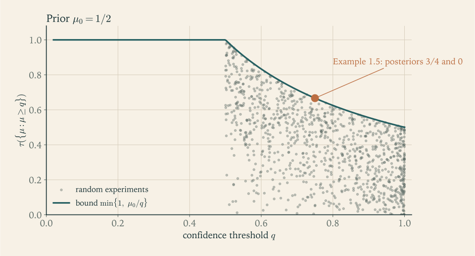
Figure 1.3 shows the bound as a frontier. Each grey point comes from an experiment drawn at random, with between two and four realizations; for each posterior \(q\) above the prior that it produces, the point records \(q\) and the probability that the posterior is at least \(q\) . None crosses the curve, and the points that come closest belong to experiments whose lowest posterior is near \(0\) , as the equality condition of Proposition 1.10 predicts. Exercise 1.10 proves the mirror-image bound for unconfident beliefs, and Exercise 1.15 generalizes the argument to ask how often an experiment can produce one particular posterior.
1.7 Tests run in sequence
Information often arrives in stages. A recruiter reads the transcript and then interviews some candidates; a regulator runs a stress test and then examines the banks that failed it. Each stage is an experiment, and the stages can be combined into one.
Let \(\pi=(S,\{\pi(\cdot\mid\omega)\})\) be a first experiment, and for each realization \(s\) let \(\pi'(\cdot\mid\omega,s)\) be a distribution on a finite set \(R\) of second-stage realizations. The second stage may depend on the first realization, which covers the recruiter who interviews only some candidates. Write \(\pi\circ\pi'\) for the composite experiment, read “\(\pi\) then \(\pi'\) ”, whose realizations are the pairs \((s,r)\) and whose likelihoods are \(\pi(s\mid\omega)\,\pi'(r\mid\omega,s)\) . For a belief \(\mu\) and a realization \(s\) , write \(\pi'_s(r\mid\mu)=\sum_\omega\mu(\omega)\pi'(r\mid\omega,s)\) for the probability of \(r\) under the second stage when the belief is \(\mu\) .
Proposition 1.11 (composition). Let \(\mu_0\) be a prior, \(\pi\) a first experiment, and \(\pi'\) a second stage as above.
(a) For every pair \((s,r)\) of positive probability, the composite posterior is the Bayes update of \(\mu_s\) by the second stage:
(b) Let \(\tau_s\) be the distribution of posteriors of the second stage \(\pi'(\cdot\mid\cdot,s)\) under the prior \(\mu_s\) . Then \(\tau_{\pi\circ\pi'}=\sum_{s:\ \pi(s)>0}\pi(s)\,\tau_s\) , each \(\tau_s\) is Bayes plausible for \(\mu_s\) , and the beliefs \(\mu_0\) , \(\mu_s\) , \(\mu_{s,r}\) form a martingale.
(c) Conversely, if for each \(s\) with \(\pi(s)>0\) the distribution \(\tau_s\) is any finite-support distribution that is Bayes plausible for \(\mu_s\) , there is a second stage \(\pi'\) with \(\tau_{\pi\circ\pi'}=\sum_s\pi(s)\,\tau_s\) .
Proof. (a) The pair \((s,r)\) has probability \(\sum_\omega\mu_0(\omega)\pi(s\mid\omega)\pi'(r\mid\omega,s)=\pi(s)\sum_\omega\mu_s(\omega)\pi'(r\mid\omega,s)=\pi(s)\,\pi'_s(r\mid\mu_s)\) , using \(\mu_0(\omega)\pi(s\mid\omega)=\pi(s)\mu_s(\omega)\) . Dividing the joint probability \(\pi(s)\mu_s(\omega)\pi'(r\mid\omega,s)\) of \(\omega\) and \((s,r)\) by this gives the formula.
(b) By (a), the posterior after \((s,r)\) is the posterior that the second stage produces from the prior \(\mu_s\) after \(r\) , and the pair has probability \(\pi(s)\) times the probability of \(r\) under that prior. Grouping pairs by their posterior, \(\tau_{\pi\circ\pi'}(\mu)=\sum_s\pi(s)\sum_{r:\ \mu_{s,r}=\mu}\pi'_s(r\mid\mu_s)=\sum_s\pi(s)\tau_s(\mu)\) . Each \(\tau_s\) is the distribution of posteriors of an experiment under the prior \(\mu_s\) , so it is Bayes plausible for \(\mu_s\) by Proposition 1.3; that says \(E[\mu_{s,r}\mid s]=\mu_s\) , and together with \(E[\mu_s]=\mu_0\) this is the martingale property.
(c) For each \(s\) , Corollary 1.5 applied with the prior \(\mu_s\) , which need not have full support, gives an experiment \(\pi'(\cdot\mid\cdot,s)\) whose distribution of posteriors under \(\mu_s\) is \(\tau_s\) . Use it as the second stage after \(s\) , choosing a common finite realization set \(R\) large enough for all \(s\) . Part (b) gives the conclusion.
Part (b) shows that sequential testing produces nothing beyond what a single experiment produces: the composite is one experiment, so its distribution of posteriors is Bayes plausible. Part (c) is the form in which composition is used later. Starting from any Bayes-plausible distribution, one may split any of its posteriors further, in any Bayes-plausible way relative to that posterior, and the result is again a feasible distribution. Chapter 6 uses this move to derive a local condition for optimality: at an optimal distribution of posteriors, no posterior in the support can be split, in a Bayes-plausible way relative to itself, so as to raise the sender’s expected payoff. Chapter 2 will add that the composite is always at least as informative as the first stage, in the sense of Blackwell (1953).
Example 1.6: An interview after the transcript
Take the two-grade transcript of Example 1.1, with posteriors \(\mu_D=2/3\) and \(\mu_P=2/11\) . A recruiter interviews only candidates with a Distinction. The interview is passed by every able candidate and by half of the others; a Pass candidate is not interviewed.
Second stage after a Distinction. Under the belief \(2/3\) , the interview is passed with probability \(\tfrac23+\tfrac13\cdot\tfrac12=\tfrac56\) . By Proposition 1.11(a) the posterior after passing is \(\tfrac23\big/\tfrac56=\tfrac45\) , and after failing it is \(0\) , since able candidates never fail. As Proposition 1.11(b) requires, \(\tfrac56\cdot\tfrac45+\tfrac16\cdot 0=\tfrac23\) .
Composite distribution. The posterior \(4/5\) has probability \(\tfrac{9}{20}\cdot\tfrac56=\tfrac38\) , the posterior \(0\) has probability \(\tfrac{9}{20}\cdot\tfrac16=\tfrac{3}{40}\) , and the posterior \(2/11\) keeps probability \(\tfrac{11}{20}\) . These sum to \(\tfrac{15}{40}+\tfrac{3}{40}+\tfrac{22}{40}=1\) , and the mean is \(\tfrac38\cdot\tfrac45+\tfrac{11}{20}\cdot\tfrac2{11}=\tfrac3{10}+\tfrac1{10}=\tfrac25\) , the prior.
As one experiment. The composite has three realizations of positive probability: Distinction and pass, Distinction and fail, and Pass. Their likelihoods are \(\bigl(\tfrac34,0,\tfrac14\bigr)\) for an able graduate and \(\bigl(\tfrac18,\tfrac18,\tfrac34\bigr)\) for any other. Directly, the first has probability \(\tfrac25\cdot\tfrac34+\tfrac35\cdot\tfrac18=\tfrac38\) and posterior \(\tfrac3{10}\big/\tfrac38=\tfrac45\) , in agreement with the two-stage calculation.
The interview split the Distinction posterior and left the Pass posterior alone. Figure 1.1 would now show three masses where it showed two, still balanced at \(2/5\) .
1.8 When only the average state matters
In many problems the state is a number, the value of an asset or the size of tomorrow’s demand, and the reader of the signal cares only about its expected value. Let \(\Omega\) be a finite set of real numbers. The posterior mean after the realization \(s\) is \(m_s=E_{\mu_s}[\omega]=\sum_\omega\mu_s(\omega)\,\omega\) . Since \(m_s\) is a linear function of the posterior, Proposition 1.3 gives
the posterior mean averages to the prior mean. A risk-neutral investor valuing an asset, a buyer deciding what a good is worth, and a driver comparing expected earnings across zones all respond only to \(m_s\) . For them, the relevant summary of an experiment is the distribution of the posterior mean, which is coarser than \(\tau\) : with three or more states, different distributions of posteriors can share one distribution of posterior means.
Which distributions of the posterior mean are achievable? The average must be the prior mean, but that is no longer enough. Full disclosure makes the posterior mean equal to the state, so its distribution is the prior distribution of \(\omega\) ; no disclosure collapses it to a point at the prior mean. Every experiment lies between, in a sense Chapter 8 makes precise. The distribution of the posterior mean is always less dispersed than the prior distribution of the state in the convex order: \(E[\varphi(m_s)]\le E_{\mu_0}[\varphi(\omega)]\) for every convex function \(\varphi\) , which follows from Jensen’s inequality applied to each posterior and then averaged. A distribution related to the prior distribution of the state in this way is called a mean-preserving contraction of it. Chapter 8 proves a converse: every finitely supported mean-preserving contraction is the distribution of the posterior mean of some finite experiment, and once experiments may have infinitely many realizations every mean-preserving contraction is achievable. Gentzkow and Kamenica (2016), building on Kolotilin (2014), used this description to solve persuasion problems in which only the mean matters. Exercise 1.17 proves one consequence, that the variance of the posterior mean never exceeds the variance of the state.
Example 1.7: Surge alerts on a ride-hailing platform
A ride-hailing platform observes the demand state of a district before its drivers do. The district is quiet, normal, or in surge, with prior probabilities \((\tfrac12,\tfrac13,\tfrac16)\) , and the corresponding numbers of unserved requests per ten minutes are \(\omega=0\) , \(3\) , and \(12\) . The prior mean is \(0+1+2=3\) . A driver nearby relocates to the district when her expected number of unserved requests is at least \(5\) , which covers her cost of moving. The platform commits to an alert policy.
Full disclosure. Posterior means are \(0\) , \(3\) , \(12\) with probabilities \(\tfrac12,\tfrac13,\tfrac16\) . Drivers relocate only in a surge, with probability \(\tfrac16\) .
Surge-only alert. An alert reveals a surge, with posterior mean \(12\) and probability \(\tfrac16\) . Without an alert the posterior is \(\bigl(\tfrac12,\tfrac13,0\bigr)\big/\tfrac56=\bigl(\tfrac35,\tfrac25,0\bigr)\) , with mean \(\tfrac25\cdot 3=\tfrac65\) . Check: \(\tfrac16\cdot 12+\tfrac56\cdot\tfrac65=2+1=3\) . Drivers relocate with probability \(\tfrac16\) .
Busy alert. An alert is sent in normal and surge states. Its posterior is \(\bigl(0,\tfrac23,\tfrac13\bigr)\) with mean \(2+4=6\) and probability \(\tfrac12\) ; without it the district is known to be quiet. Drivers relocate with probability \(\tfrac12\) .
The ceiling. The posterior mean is nonnegative and averages \(3\) , so Markov’s inequality, exactly as in the proof of Proposition 1.10, gives \(\Pr(m_s\ge 5)\le\tfrac35\) . Equality requires every posterior mean to be \(0\) or \(5\) , and a posterior mean of \(0\) requires certainty that the district is quiet. One policy that attains the ceiling sends an alert in every normal or surge state and with probability \(\alpha\) in a quiet one; it is not the only one, since any policy whose posterior means are all \(0\) or \(5\) does as well. The alert’s posterior mean is \(3\big/\bigl(\tfrac12+\tfrac12\alpha\bigr)\) , which equals \(5\) when \(\alpha=\tfrac15\) . The alert then has probability \(\tfrac13+\tfrac16+\tfrac1{10}=\tfrac35\) and posterior \(\bigl(\tfrac16,\tfrac59,\tfrac5{18}\bigr)\) , whose mean is \(\tfrac59\cdot 3+\tfrac5{18}\cdot 12=5\) .
The four policies show the trade-off that the rest of the course formalizes. Revealing more does not mean moving more drivers: full disclosure moves drivers a sixth of the time, while the ceiling policy, which hides the difference between normal and surge and sometimes alerts in a quiet district, moves them three times in five. Whether the platform should want that depends on what drivers who arrive in a quiet district cost it, and with many drivers deciding at once, on how they crowd one another. Those questions belong to Chapters 6 and 9.
1.9 Where the change of variables leads
The chapter has replaced experiments by distributions of posteriors and shown that the replacement is exact: Corollary 1.5 says which distributions are feasible, Proposition 1.7 says what the replacement forgets, and Propositions 1.9 to 1.11 give the geometry, the limits on confidence, and the rules for combining tests. Three directions lead from here.
The first asks what information is worth to the person who receives it. A decision maker’s best expected payoff at a belief is a convex function of the belief, and Chapter 2 shows that this convexity, together with Proposition 1.9, makes information valuable and lets one experiment be ranked above another for every decision maker at once, which is the theorem of Blackwell (1953).
The second asks what a sender who controls the experiment should choose. Suppose her expected payoff when the receiver holds the posterior \(\mu\) is \(\hat v(\mu)\) , and let \(V\) be the concave envelope of \(\hat v\) , the smallest concave function that lies above it. Chapter 6 proves that the supremum of the sender’s expected payoff over all experiments is \(V(\mu_0)\) , and that it is attained whenever \(\hat v\) is upper semicontinuous, which holds when the receiver has finitely many actions and breaks ties in the sender’s favour. This is the concavification theorem of Kamenica and Gentzkow (2011), and Proposition 1.9 is its first half. Chapters 3 to 5 first study senders who cannot commit to an experiment, for whom the feasible distributions of posteriors are smaller.
The third asks what survives when the simple picture of this chapter breaks. With infinitely many states, finitely many target posteriors still need only densities (Exercise 1.19), but a target with a continuum of posteriors needs regular conditional distributions, the measure-theoretic tools of Chapter 8. With several receivers who see different signals, one receiver’s distribution of posteriors no longer describes what the designer has done, because each receiver also forms beliefs about what the others believe; Chapter 9 replaces distributions of posteriors by Bayes correlated equilibria. For surveys of the field that this course follows, see Bergemann and Morris (2019) and Kamenica (2019).
Exercises
-
State Definition 1.2 and Proposition 1.3 from memory, then explain in two or three sentences why the formula of Theorem 1.4 divides by \(\mu_0(\omega)\) , what goes wrong with that formula when some state has prior probability zero, and how the proof of Corollary 1.5 repairs it.
Answer
Definition 1.2 and Proposition 1.3 are stated in Sections 1.2 and 1.3. The formula \(\pi(\mu\mid\omega)=\tau(\mu)\mu(\omega)/\mu_0(\omega)\) divides by the prior because it turns the target joint probability \(\tau(\mu)\mu(\omega)\) of a state and a realization into a probability conditional on the state. If \(\mu_0(\omega)=0\) the quotient is undefined. Bayes plausibility then forces \(\mu(\omega)=0\) for every posterior in the support, so the joint probabilities in that state’s row are all zero and the row carries no information; the proof of Corollary 1.5 fills it with an arbitrary distribution, which never affects a realization probability or a posterior.
-
A binary state has prior \(\mu_0=1/4\) and an experiment with realizations \(h\) , \(k\) , \(\ell\) whose likelihoods are \(\pi(h\mid 1)=1/2\) , \(\pi(k\mid 1)=1/3\) , \(\pi(\ell\mid 1)=1/6\) , \(\pi(h\mid 0)=1/6\) , \(\pi(k\mid 0)=1/3\) , \(\pi(\ell\mid 0)=1/2\) . Compute \(\pi(s)\) and \(\mu_s\) for each realization, write \(\tau_\pi\) , verify Proposition 1.3, and explain why one realization leaves the belief at the prior.
Solution
Write the joint probabilities \(\mu_0(\omega)\pi(s\mid\omega)\) first. With \(\mu_0=1/4\) , the state \(\omega=1\) contributes \(\tfrac14\cdot\tfrac12=\tfrac18\) , \(\tfrac14\cdot\tfrac13=\tfrac1{12}\) , \(\tfrac14\cdot\tfrac16=\tfrac1{24}\) to \(h\) , \(k\) , \(\ell\) , and the state \(\omega=0\) contributes \(\tfrac34\cdot\tfrac16=\tfrac18\) , \(\tfrac34\cdot\tfrac13=\tfrac14\) , \(\tfrac34\cdot\tfrac12=\tfrac38\) . Adding each column,
\[ \pi(h)=\tfrac18+\tfrac18=\tfrac14,\qquad \pi(k)=\tfrac1{12}+\tfrac14=\tfrac13,\qquad \pi(\ell)=\tfrac1{24}+\tfrac38=\tfrac5{12}. \]The posteriors are the \(\omega=1\) entries divided by the column totals:
\[ \mu_h=\frac{1/8}{1/4}=\frac12,\qquad \mu_k=\frac{1/12}{1/3}=\frac14,\qquad \mu_\ell=\frac{1/24}{5/12}=\frac1{10}. \]The three posteriors are distinct, so \(\tau_\pi(1/2)=1/4\) , \(\tau_\pi(1/4)=1/3\) , \(\tau_\pi(1/10)=5/12\) . Proposition 1.3 holds:
\[ \tfrac14\cdot\tfrac12+\tfrac13\cdot\tfrac14+\tfrac5{12}\cdot\tfrac1{10}=\tfrac{3}{24}+\tfrac{2}{24}+\tfrac{1}{24}=\tfrac14 . \]The realization \(k\) has the same likelihood \(1/3\) in both states, so its likelihood ratio is \(1\) . In odds form, the posterior odds equal the prior odds times one, and the belief after \(k\) is the prior \(1/4\) . A realization that is equally likely in every state carries no information, however often it occurs.
-
With \(\omega=1\) meaning the able or strong type, recast as distributions of posteriors (a) the separating equilibrium of Game Theory Example 8.2, (b) the pooling equilibrium on \(N\) of the same example, and (c) the partially separating equilibrium of Game Theory Exercise 8.8, in which the bet is \(2\) ; verify Bayes plausibility in each case and say which one is the distribution of full disclosure.
Solution
Let \(\omega=1\) be the able type in Game Theory Example 8.2, where the prior is \(1/2\) .
(a) In the separating equilibrium the able type obtains the degree and the other type does not; as in Game Theory, \(D\) and \(N\) here denote obtaining the degree or not, not the grades of Example 1.1. As an experiment, \(\pi(D\mid 1)=1\) and \(\pi(N\mid 0)=1\) . Each message has probability \(1/2\) , the posterior after \(D\) is \(1\) , and after \(N\) it is \(0\) . So \(\tau(1)=\tfrac12\) and \(\tau(0)=\tfrac12\) , with mean \(\tfrac12\) . This is the distribution of full disclosure.
(b) In the pooling equilibrium both types choose \(N\) , so the experiment has one realization of positive probability, and its posterior is the prior. The distribution is the point mass \(\tau(1/2)=1\) , which trivially averages to \(1/2\) . The off-path message \(D\) has probability zero and does not enter \(\tau\) .
(c) In Game Theory Exercise 8.8 the bet is \(2\) , so a called bet wins or loses \(3\) while a fold loses the stake \(1\) . High always bets. Low must bluff with some probability \(\beta\in(0,1)\) by the argument of Game Theory Example 8.4, and the receiver must be indifferent after a bet. If his belief in High after a bet is \(\mu\) , calling yields \(-3\mu+3(1-\mu)=3-6\mu\) and folding yields \(-1\) , so indifference requires \(\mu=2/3\) . By Bayes’ rule \(\mu=\tfrac12\big/\bigl(\tfrac12+\tfrac12\beta\bigr)=1/(1+\beta)\) , so \(\beta=1/2\) . As an experiment, \(\pi(\mathrm{Bet}\mid 1)=1\) and \(\pi(\mathrm{Bet}\mid 0)=\tfrac12\) . A bet has probability \(\tfrac12+\tfrac14=\tfrac34\) and posterior \(2/3\) ; a fold has probability \(\tfrac14\) and posterior \(0\) . Thus \(\tau(2/3)=\tfrac34\) , \(\tau(0)=\tfrac14\) , and \(\tfrac34\cdot\tfrac23+\tfrac14\cdot 0=\tfrac12\) . The posteriors move away from the prior without both becoming certain, the mark of partial separation.
-
A school’s brochure claims that a well-designed test can make every employer more confident that a graduate is able, because the school can choose grades so that every grade raises the employer’s belief above the prior; find the error, and prove that if some realization of positive probability has \(\mu_s(\omega)>\mu_0(\omega)\) , then another realization of positive probability has \(\mu_s(\omega)<\mu_0(\omega)\) .
Solution
The brochure’s claim is that one can choose grades so that every grade, or at least every grade that is ever awarded, leaves the employer with a belief above the prior. Proposition 1.3 rules this out. Fix the state \(\omega\) in which the graduate is able. Subtracting \(\mu_0(\omega)=\sum_s\pi(s)\mu_0(\omega)\) from both sides of the identity \(\sum_{s:\ \pi(s)>0}\pi(s)\mu_s(\omega)=\mu_0(\omega)\) gives
\[ \sum_{s:\ \pi(s)>0}\pi(s)\bigl(\mu_s(\omega)-\mu_0(\omega)\bigr)=0 . \]Suppose some realization \(s^\ast\) with \(\pi(s^\ast)>0\) has \(\mu_{s^\ast}(\omega)>\mu_0(\omega)\) . Its term in the sum is strictly positive. A sum of terms equal to zero that contains a strictly positive term must contain a strictly negative one, so some realization \(s'\) with \(\pi(s')>0\) has \(\mu_{s'}(\omega)<\mu_0(\omega)\) . Every grade that makes some graduates look better is paid for by a grade that makes others look worse, and the probability-weighted gains and losses cancel exactly. The error in the brochure is to think of each grade separately; the beliefs it produces are tied together because they are all conditional probabilities computed from one joint distribution whose state marginal is the prior.
-
Prove that under any experiment the expected posterior probability of the true state, \(\sum_\omega\sum_{s:\,\pi(s)>0}\mu_0(\omega)\pi(s\mid\omega)\mu_s(\omega)\) , is at least \(\sum_\omega\mu_0(\omega)^2\) , with equality exactly when every posterior of positive probability equals the prior, and explain why this does not contradict Proposition 1.3.
Solution
The sum runs over realizations of positive probability, the only ones whose posteriors are defined and the only ones ever observed. Because \(\mu_0(\omega)\pi(s\mid\omega)=\pi(s)\mu_s(\omega)\) for each such realization, the expected posterior probability of the true state is
\[ \sum_\omega\sum_{s:\ \pi(s)>0}\mu_0(\omega)\pi(s\mid\omega)\mu_s(\omega)=\sum_{s:\ \pi(s)>0}\pi(s)\sum_\omega\mu_s(\omega)^2=E_\tau\Bigl[\sum_\omega\mu(\omega)^2\Bigr]. \]For each \(\omega\) , expand the square around the prior and use \(E_\tau[\mu(\omega)]=\mu_0(\omega)\) from Proposition 1.3:
\[ E_\tau\bigl[\mu(\omega)^2\bigr]=\mu_0(\omega)^2+E_\tau\bigl[(\mu(\omega)-\mu_0(\omega))^2\bigr], \]because the cross term \(2\mu_0(\omega)E_\tau[\mu(\omega)-\mu_0(\omega)]\) is zero. Summing over \(\omega\) ,
\[ E_\tau\Bigl[\sum_\omega\mu(\omega)^2\Bigr]=\sum_\omega\mu_0(\omega)^2+E_\tau\Bigl[\sum_\omega(\mu(\omega)-\mu_0(\omega))^2\Bigr]\ge\sum_\omega\mu_0(\omega)^2 . \]The last expectation is a weighted sum, with positive weights, of nonnegative numbers, so it is zero exactly when every posterior in the support equals \(\mu_0\) . There is no contradiction with Proposition 1.3. That proposition fixes the expected probability of each given state. The quantity here is the probability assigned to the state that actually occurred, which varies with the state; experiments raise it because high posteriors on \(\omega\) occur disproportionately when \(\omega\) is the truth.
-
For a binary state with prior \(\mu_0\) and target posteriors \(\mu_L<\mu_0<\mu_H\) , derive closed forms for the two likelihoods \(\pi(\mu_H\mid 1)\) and \(\pi(\mu_H\mid 0)\) of the direct experiment that induces them, check that both lie in \([0,1]\) exactly because \(\mu_L\le\mu_0\le\mu_H\) , and evaluate them for \(\mu_0=1/3\) , \(\mu_L=1/10\) , \(\mu_H=3/5\) , verifying both posteriors by Bayes’ rule.
Solution
Write \(H\) for the realization whose posterior is \(\mu_H\) . By Proposition 1.8(b), \(\tau(\mu_H)=(\mu_0-\mu_L)/(\mu_H-\mu_L)\) , and Theorem 1.4 gives \(\pi(\mu_H\mid\omega)=\tau(\mu_H)\mu_H(\omega)/\mu_0(\omega)\) , where \(\mu_H(1)=\mu_H\) and \(\mu_H(0)=1-\mu_H\) . Hence
\[ \pi(\mu_H\mid 1)=\frac{\mu_H(\mu_0-\mu_L)}{\mu_0(\mu_H-\mu_L)},\qquad \pi(\mu_H\mid 0)=\frac{(1-\mu_H)(\mu_0-\mu_L)}{(1-\mu_0)(\mu_H-\mu_L)} . \]Both are nonnegative exactly when \(\mu_0\ge\mu_L\) . The first is at most one exactly when \(\mu_H\mu_0-\mu_H\mu_L\le\mu_0\mu_H-\mu_0\mu_L\) , that is, \(\mu_L(\mu_H-\mu_0)\ge 0\) , which holds because \(\mu_H\ge\mu_0\) . The second is at most one exactly when \((1-\mu_H)(\mu_0-\mu_L)\le(1-\mu_0)(\mu_H-\mu_L)\) ; expanding and cancelling, this is \(\mu_0(1-\mu_L)\le\mu_H(1-\mu_L)\) , again \(\mu_0\le\mu_H\) . So the region of valid targets is exactly \(\mu_L\le\mu_0\le\mu_H\) .
With \(\mu_0=1/3\) , \(\mu_L=1/10\) , \(\mu_H=3/5\) : \(\tau(\mu_H)=\tfrac{7/30}{1/2}=\tfrac7{15}\) , and
\[ \pi(\mu_H\mid 1)=\frac{\tfrac35\cdot\tfrac7{30}}{\tfrac13\cdot\tfrac12}=\frac{21}{25},\qquad \pi(\mu_H\mid 0)=\frac{\tfrac25\cdot\tfrac7{30}}{\tfrac23\cdot\tfrac12}=\frac{7}{25}. \]Check by Bayes’ rule. The high realization has probability \(\tfrac13\cdot\tfrac{21}{25}+\tfrac23\cdot\tfrac7{25}=\tfrac{7}{25}+\tfrac{14}{75}=\tfrac{7}{15}\) and posterior \(\tfrac{7/25}{7/15}=\tfrac35\) . The low realization has likelihoods \(\tfrac4{25}\) and \(\tfrac{18}{25}\) , probability \(\tfrac{4}{75}+\tfrac{36}{75}=\tfrac{8}{15}\) , and posterior \(\tfrac{4/75}{8/15}=\tfrac1{10}\) .
-
With three equally likely states, let \(\tau\) put probability \(1/3\) on each of \((\tfrac12,\tfrac12,0)\) , \((0,\tfrac12,\tfrac12)\) , and \((\tfrac12,0,\tfrac12)\) ; check that \(\tau\) is Bayes plausible, construct the experiment of Theorem 1.4, and describe in one plain sentence what this experiment tells its reader about the state.
Answer
The weights average to \((\tfrac13,\tfrac13,\tfrac13)\) , so \(\tau\) is Bayes plausible. Since \(\tau(\mu)=\mu_0(\omega)=1/3\) , the construction gives \(\pi(\mu\mid\omega)=\mu(\omega)\) : in state \(\omega_1\) the realizations \((\tfrac12,\tfrac12,0)\) and \((\tfrac12,0,\tfrac12)\) each have probability \(1/2\) , and similarly in the other states. In words, the experiment names one of the two false states, chosen at random with equal probability, and rules it out.
-
A binary state has prior \(0.6\) , and a consultant proposes posteriors \(0.8\) and \(0.5\) with probability \(1/2\) each; show that no experiment induces this proposal, find the unique Bayes-plausible distribution on \(\{0.5,0.8\}\) , find all Bayes-plausible distributions on \(\{0,0.5,0.8\}\) , and explain with Proposition 1.8 why uniqueness fails for the larger support.
Solution
The proposal averages to \(\tfrac12\cdot 0.8+\tfrac12\cdot 0.5=0.65\) , not the prior \(0.6\) , so by Proposition 1.3 no experiment induces it. On \(\{0.5,0.8\}\) , two distinct numbers on either side of \(0.6\) , Proposition 1.8(b) gives the unique Bayes-plausible weights
\[ \tau(0.8)=\frac{0.6-0.5}{0.8-0.5}=\frac13,\qquad \tau(0.5)=\frac23 . \]On \(\{0,0.5,0.8\}\) , write the weights as \(a\) , \(b\) , \(c\) . Bayes plausibility and total mass give \(0.5b+0.8c=0.6\) and \(a+b+c=1\) , so \(b=1.2-1.6c\) and \(a=1-b-c=0.6c-0.2\) . Nonnegativity requires \(b\ge 0\) , so \(c\le\tfrac34\) , and \(a\ge 0\) , so \(c\ge\tfrac13\) . Every \(c\in[\tfrac13,\tfrac34]\) works, giving a one-parameter family that runs from the distribution with \(a=0\) found above to the distribution \(\tau(0.8)=\tfrac34\) , \(\tau(0)=\tfrac14\) , with \(b=0\) . Uniqueness fails because Proposition 1.8(a) requires affinely independent posteriors. In the binary case the simplex is a segment of affine dimension one, so at most two beliefs can be affinely independent, and three beliefs on a line can balance at the prior in infinitely many ways.
-
An online marketplace knows that a fifth of its sellers are low quality, and buyers avoid any seller whose posterior probability of being low quality is at least \(2/3\) ; find the largest fraction of sellers that a committed flagging policy can make buyers avoid, a policy that attains it, and the posterior attached to sellers who are not flagged.
Solution
Let the state of interest be that the seller is low quality, with prior probability \(\mu_0(\text{low})=\tfrac15\) , and let \(q=\tfrac23\) . A seller is avoided exactly when her posterior probability of low quality is at least \(q\) . By Proposition 1.10 the fraction avoided under any committed flagging policy is at most
\[ \frac{\mu_0(\text{low})}{q}=\frac{1/5}{2/3}=\frac{3}{10}. \]Since \(\tfrac15\le\tfrac23\) , the bound is attained, and the construction in the proof of Proposition 1.10 shows how. Flag every low-quality seller, and flag a high-quality seller with probability
\[ \beta=\frac{\tfrac15\bigl(1-\tfrac23\bigr)}{\tfrac23\cdot\tfrac45}=\frac{1/15}{8/15}=\frac18 . \]A flag then has probability \(\tfrac15+\tfrac45\cdot\tfrac18=\tfrac3{10}\) , and the posterior probability of low quality after a flag is \(\tfrac{1/5}{3/10}=\tfrac23\) , exactly the buyers’ threshold, so every flagged seller is avoided. Unflagged sellers are certainly high quality: their posterior probability of low quality is \(0\) . Any policy that avoids \(3/10\) of sellers must, by the equality condition, put every seller at posterior \(0\) or \(2/3\) .
-
Prove that for every experiment, every state \(\omega\) , and every \(r\in[0,1)\) , \(\tau_\pi(\{\mu:\mu(\omega)\le r\})\le(1-\mu_0(\omega))/(1-r)\) , determine when equality holds, and construct an attaining experiment for a binary state with \(\mu_0=1/2\) and \(r=1/5\) .
Hint
Apply Proposition 1.10 to the event \(E=\Omega\setminus\{\omega\}\) , whose prior probability is \(1-\mu_0(\omega)\) , with the threshold \(1-r\) ; a posterior satisfies \(\mu(\omega)\le r\) exactly when \(\mu(E)\ge 1-r\) . If \(E\) is empty, the bound is trivial.
Answer
When \(r\le\mu_0(\omega)\) , equality holds exactly when every posterior gives \(\omega\) probability \(r\) or \(1\) . For \(\mu_0=1/2\) and \(r=1/5\) the bound is \(5/8\) : send the realization doubt always when \(\omega=0\) and with probability \(1/4\) when \(\omega=1\) ; it has probability \(5/8\) and posterior \(1/5\) , and the other realization has posterior \(1\) .
-
Assuming the prior has full support, prove that two realizations \(s\) and \(s'\) of positive probability produce the same posterior if and only if their likelihood vectors are proportional, \(\pi(s\mid\cdot)=c\,\pi(s'\mid\cdot)\) for some \(c>0\) , and use this to explain why grades A and B were merged in Example 1.1.
Hint
Write the posterior as \(\mu_s(\omega)=\mu_0(\omega)\pi(s\mid\omega)/\pi(s)\) . If the likelihoods are proportional with constant \(c\) , then so are the column totals, and the constant cancels. Conversely, if \(\mu_s=\mu_{s'}\) , solve both expressions for the likelihood and divide; full support lets you cancel \(\mu_0(\omega)\) . In Example 1.1 the likelihood vectors of A and B are \((\tfrac16,\tfrac12)\) and \((\tfrac1{12},\tfrac14)\) in the order \((\omega=0,\omega=1)\) , with \(c=2\) .
-
A binary state has prior \(1/2\) , and an experiment with \(\pi(h\mid 1)=\pi(\ell\mid 0)=2/3\) is run twice, the two runs independent given the state; compute the distribution of posteriors after both runs in two ways, by updating twice with Proposition 1.11 and as one experiment with four realizations, and verify that the beliefs form a martingale.
Solution
Updating twice. The first run has \(\pi(h)=\tfrac12\cdot\tfrac23+\tfrac12\cdot\tfrac13=\tfrac12\) , with posterior \(\mu_h=2/3\) , and \(\pi(\ell)=\tfrac12\) , with posterior \(\mu_\ell=1/3\) . By Proposition 1.11(a) the second run updates these beliefs. From \(2/3\) , a second \(h\) has probability \(\tfrac23\cdot\tfrac23+\tfrac13\cdot\tfrac13=\tfrac59\) and gives the posterior \(\tfrac{4/9}{5/9}=\tfrac45\) ; a second \(\ell\) has probability \(\tfrac49\) and gives \(\tfrac{2/9}{4/9}=\tfrac12\) . From \(1/3\) , a second \(h\) has probability \(\tfrac49\) and gives \(\tfrac12\) ; a second \(\ell\) has probability \(\tfrac59\) and gives \(\tfrac{1/9}{5/9}=\tfrac15\) . By Proposition 1.11(b),
\[ \tau(4/5)=\tfrac12\cdot\tfrac59=\tfrac5{18},\qquad \tau(1/2)=\tfrac12\cdot\tfrac49+\tfrac12\cdot\tfrac49=\tfrac49,\qquad \tau(1/5)=\tfrac12\cdot\tfrac59=\tfrac5{18}. \]As one experiment. The four realizations \(hh\) , \(h\ell\) , \(\ell h\) , \(\ell\ell\) have likelihoods \(\tfrac49,\tfrac29,\tfrac29,\tfrac19\) when \(\omega=1\) and \(\tfrac19,\tfrac29,\tfrac29,\tfrac49\) when \(\omega=0\) . Their probabilities are \(\tfrac5{18},\tfrac29,\tfrac29,\tfrac5{18}\) , and their posteriors are \(\tfrac{2/9}{5/18}=\tfrac45\) , \(\tfrac12\) , \(\tfrac12\) , and \(\tfrac{1/18}{5/18}=\tfrac15\) . Merging \(h\ell\) and \(\ell h\) reproduces the distribution above.
Martingale. After the first \(h\) , the expected second-stage posterior is \(\tfrac59\cdot\tfrac45+\tfrac49\cdot\tfrac12=\tfrac23\) ; after the first \(\ell\) it is \(\tfrac49\cdot\tfrac12+\tfrac59\cdot\tfrac15=\tfrac13\) ; and the first-stage posteriors average to \(\tfrac12\cdot\tfrac23+\tfrac12\cdot\tfrac13=\tfrac12\) . Each belief is the expectation of the next one.
-
Using Proposition 1.11, show that a recruiter who has already seen the transcript of Example 1.1 can reach full disclosure with a suitable second stage, but cannot reach the distribution with posteriors \(3/5\) and \(0\) that Example 1.5 constructed to make as many graduates as possible look at least \(60\) percent likely to be able, and explain in one sentence why information once revealed cannot be withdrawn.
Solution
By Proposition 1.11(b) and (c), a second stage after the transcript can produce exactly the distributions \(\tfrac9{20}\tau_D+\tfrac{11}{20}\tau_P\) in which \(\tau_D\) is Bayes plausible for the belief \(\mu_D=2/3\) and \(\tau_P\) is Bayes plausible for \(\mu_P=2/11\) .
Full disclosure is reachable. Split \(2/3\) into the posteriors \(1\) and \(0\) with weights \(2/3\) and \(1/3\) , and split \(2/11\) into \(1\) and \(0\) with weights \(2/11\) and \(9/11\) ; both splits are Bayes plausible by Proposition 1.8(b). The composite puts \(\tfrac9{20}\cdot\tfrac23+\tfrac{11}{20}\cdot\tfrac2{11}=\tfrac25\) on the posterior \(1\) and \(\tfrac35\) on the posterior \(0\) , which is full disclosure. A second stage that simply reveals the state does this.
The distribution of Example 1.5 is not reachable. The target puts weight \(2/3\) on \(3/5\) and \(1/3\) on \(0\) . A composite equal to it would have every \(\tau_s\) supported in \(\{0,3/5\}\) . But \(\tau_D\) must average to \(2/3\) , and any distribution on \(\{0,3/5\}\) has mean at most \(3/5<2/3\) . So no second stage works. Once the transcript has made some candidates \(2/3\) likely to be able, later tests can only spread beliefs around \(2/3\) ; they cannot pull the candidates back to the less confident \(3/5\) , because information once revealed cannot be withdrawn.
-
A student wants posteriors \(0.9\) and \(0.1\) from the prior \(0.2\) and proposes the experiment that sends “high” with probability \(0.9\) when \(\omega=1\) and \(0.1\) when \(\omega=0\) , reasoning that each realization should be drawn with the probabilities of its posterior; compute the posteriors this experiment really produces, locate the error relative to Theorem 1.4, give the correct experiment, and explain why the student’s rule happens to work at the prior \(1/2\) .
Solution
With prior \(0.2\) , the student’s experiment has \(\Pr(\text{high})=0.2\cdot 0.9+0.8\cdot 0.1=0.26\) and posterior
\[ \mu_{\text{high}}=\frac{0.18}{0.26}=\frac{9}{13}\approx 0.69,\qquad \mu_{\text{low}}=\frac{0.2\cdot 0.1}{0.74}=\frac{1}{37}\approx 0.027, \]not \(0.9\) and \(0.1\) . The student set \(\pi(\mu\mid\omega)=\mu(\omega)\) and dropped the factor \(\tau(\mu)/\mu_0(\omega)\) of Theorem 1.4. That factor converts the posterior, a probability of the state given the realization, into a likelihood, a probability of the realization given the state; it is the same confusion as the common mistake of Section 1.2, run in reverse. The correct weights come from Proposition 1.8(b): \(\tau(0.9)=(0.2-0.1)/(0.9-0.1)=\tfrac18\) and \(\tau(0.1)=\tfrac78\) . Theorem 1.4 then gives
\[ \pi(\text{high}\mid 1)=\frac{\tfrac18\cdot 0.9}{0.2}=\frac{9}{16},\qquad \pi(\text{high}\mid 0)=\frac{\tfrac18\cdot 0.1}{0.8}=\frac{1}{64}. \]Check: \(\Pr(\text{high})=0.2\cdot\tfrac9{16}+0.8\cdot\tfrac1{64}=0.1125+0.0125=0.125\) and the posterior is \(0.1125/0.125=0.9\) . At the prior \(1/2\) , the lever rule gives \(\tau(0.9)=\tau(0.1)=\tfrac12\) , so \(\tau(\mu)/\mu_0(\omega)=1\) for every realization and state, and the factor the student forgot happens to equal one.
-
Prove that the largest probability with which any experiment can produce one particular posterior \(\mu\) is \(\min\{\mu_0(\omega)/\mu(\omega):\mu(\omega)>0\}\) , then compute it for \(\mu_0=(\tfrac12,\tfrac3{10},\tfrac15)\) and \(\mu=(\tfrac14,\tfrac14,\tfrac12)\) and compare the answer with the watch rating of Example 1.4.
Solution
Let \(\tau\) be any Bayes-plausible distribution, and let \(\mu\) be one of its posteriors. Every term of \(\sum_{\mu'}\tau(\mu')\mu'(\omega)=\mu_0(\omega)\) is nonnegative, so the single term for \(\mu\) is at most the sum: \(\tau(\mu)\mu(\omega)\le\mu_0(\omega)\) for every \(\omega\) . Hence \(\tau(\mu)\le\mu_0(\omega)/\mu(\omega)\) whenever \(\mu(\omega)>0\) , and
\[ \tau(\mu)\le t^\ast=\min\Bigl\{\frac{\mu_0(\omega)}{\mu(\omega)}:\mu(\omega)>0\Bigr\}. \]The bound is attained. If \(t^\ast\ge 1\) , then \(\mu_0(\omega)\ge\mu(\omega)\) for all \(\omega\) , and since both sum to one, \(\mu=\mu_0\) and \(t^\ast=1\) exactly, so the printed formula gives \(1\) , which no disclosure attains. If \(t^\ast<1\) , then \(\mu\ne\mu_0\) , and the vector \(\nu=(\mu_0-t^\ast\mu)/(1-t^\ast)\) has nonnegative entries by the choice of \(t^\ast\) and sums to one, so it is a belief, with \(t^\ast\mu+(1-t^\ast)\nu=\mu_0\) . Moreover \(\nu\ne\mu\) , since \(\nu=\mu\) would give \(\mu=\mu_0\) . The distribution with weight \(t^\ast\) on \(\mu\) and \(1-t^\ast\) on the different belief \(\nu\) is Bayes plausible and gives \(\mu\) exactly the probability \(t^\ast\) , and Corollary 1.5 supplies an experiment. For \(\mu_0=(\tfrac12,\tfrac3{10},\tfrac15)\) and \(\mu=(\tfrac14,\tfrac14,\tfrac12)\) the three ratios are
\[ \frac{1/2}{1/4}=2,\qquad \frac{3/10}{1/4}=\frac65,\qquad \frac{1/5}{1/2}=\frac25, \]so the largest probability is \(\tfrac25\) , fixed by the bad state. The watch rating of Example 1.4 has exactly this probability: it already puts on watch every bad borrower, which is the binding constraint, so no rating scale could make that posterior more frequent.
-
In the three-state simplex with prior \(\mu_0=(\tfrac12,\tfrac3{10},\tfrac15)\) , find every belief \(\mu\) for which a Bayes-plausible distribution with support exactly \(\{(1,0,0),\mu\}\) exists, describe that set geometrically, and compute the two weights when \(\mu\) lies on the edge where \(\mu(G)=0\) .
Answer
Bayes plausibility with weight \(t\) on \((1,0,0)\) requires \(\mu=(\mu_0-t(1,0,0))/(1-t)\) with \(0<t\le\tfrac12\) . These beliefs form the segment from \(\mu_0\) , excluded, to \((0,\tfrac35,\tfrac25)\) , included: the part of the line through the vertex \(G\) and the prior that lies beyond the prior. On the edge \(\mu(G)=0\) the belief is \((0,\tfrac35,\tfrac25)\) and both weights are \(\tfrac12\) .
-
For a real-valued state with posterior mean \(m_s=E_{\mu_s}[\omega]\) , prove that the variance of \(m_s\) across realizations is at most the prior variance of \(\omega\) , with equality exactly when every posterior of positive probability is degenerate, and compute both variances for the surge-only alert of Example 1.7.
Hint
Use the law of total variance, \(\mathrm{Var}(\omega)=E[\mathrm{Var}(\omega\mid s)]+\mathrm{Var}(E[\omega\mid s])\) , which follows from the tower property. The first term is zero exactly when every posterior puts all its mass on one value of \(\omega\) . For the surge-only alert, the prior variance is \(27-9=18\) and the variance of the posterior mean is \(\tfrac16\cdot 144+\tfrac56\cdot\tfrac{36}{25}-9=\tfrac{81}{5}\) .
-
In Game Theory Example 7.2 a trade association commits before production to an experiment about firm 2’s cost whose realization both firms see, and firm 1’s quantity at a posterior \(\mu\) is \(q_1=(a-2c_1+E_\mu[c_2])/3\) as in Game Theory Exercise 7.6 with \(a=14\) and \(c_1=2\) ; show that firm 1’s expected quantity is \(4\) under every such experiment, as without the report, and say which step uses Proposition 1.3.
Solution
After a public realization that leads both firms to the posterior \(\mu\) about firm 2’s cost, the game is the Bayesian game of Game Theory Example 7.2 with prior \(\mu\) in place of the original prior: firm 2 still knows its cost and firm 1 knows only \(\mu\) . Game Theory Exercise 7.6 gives firm 1’s quantity in that game as
\[ q_1(\mu)=\frac{a-2c_1+E_\mu[c_2]}{3}=\frac{10+E_\mu[c_2]}{3} \]with \(a=14\) and \(c_1=2\) , assuming all quantities are positive, which holds for costs in \(\{0,4\}\) . The quantity is an affine function of the posterior mean of the cost, and the posterior mean is a linear function of the posterior. Taking expectations over the realization and using Proposition 1.3 in the form \(E_\tau[E_\mu[c_2]]=\sum_\mu\tau(\mu)\sum_cc\,\mu(c)=\sum_cc\,\mu_0(c)=E_{\mu_0}[c_2]=2\) ,
\[ E_\tau[q_1(\mu)]=\frac{10+E_\tau\bigl[E_\mu[c_2]\bigr]}{3}=\frac{10+2}{3}=4 , \]which is firm 1’s quantity without the report. For instance, full disclosure gives \(10/3\) or \(14/3\) with probability \(1/2\) each, averaging \(4\) . The step that uses Proposition 1.3 is the interchange of the average over posteriors with the average over costs. The conclusion depends on linearity: firm 1’s expected profit, which is not linear in the posterior mean, does change with the report, as Game Theory Exercise 7.18 shows.
-
The splitting construction extends to infinitely many states, a case Chapter 8 treats in general: for \(\Omega=[0,1]\) with a positive prior density \(f_0\) and finitely many target posterior densities \(f_1,\dots,f_k\) with weights \(\tau_1,\dots,\tau_k\) satisfying \(\sum_j\tau_jf_j=f_0\) , write the analogue of the formula in Theorem 1.4, check that it gives a distribution over realizations for each state, and name the step that would need a measure-theoretic argument if the target had a continuum of posteriors.
Hint
The analogue is \(\pi(j\mid\omega)=\tau_jf_j(\omega)/f_0(\omega)\) . Densities are defined only up to sets of measure zero, so \(\sum_j\tau_jf_j=f_0\) holds almost everywhere; on the exceptional null set, define \(\pi(\cdot\mid\omega)\) arbitrarily. Elsewhere, summing over \(j\) gives one. Each realization has positive probability \(\tau_j\) , so the posterior density follows from Bayes’ rule for an event of positive probability. With a continuum of target posteriors, individual realizations have probability zero, and the posterior must be defined as a regular conditional distribution, which is where conditional expectation in the measure-theoretic sense from Measure-Theoretic Probability (
math.measure-theoretic-probability.conditional-expectation) is needed; that course states the existence of regular conditional distributions without proving it. -
A ride-hailing platform faces the three demand states of Example 1.7, but its drivers relocate only when the posterior probability of a surge is at least \(1/2\) ; find the largest relocation probability any alert policy can produce and a policy attaining it, and explain why the answer differs from the ceiling in Example 1.7 although the prior is the same.
Answer
The largest relocation probability is \(\tfrac{1/6}{1/2}=\tfrac13\) . Alert in every surge and, in a quiet or normal state, with probability \(\tfrac15\) ; the alert has probability \(\tfrac16+\tfrac56\cdot\tfrac15=\tfrac13\) and posterior surge probability \(\tfrac12\) . The answer is smaller than \(\tfrac35\) because only surge probability counts now, whereas under the mean criterion a normal state contributed \(3\) unserved requests toward the threshold of \(5\) .
-
Explain to a classmate who has finished Game Theory Chapter 8 why the receiver’s posterior was a by-product of equilibrium there but is the object of choice here, which of the conditions (S), (R), and (B) of Game Theory Section 8.3 disappears when the sender commits to an experiment, and why Bayes plausibility survives every change of model in this course.
Answer
A model answer names three points. In Game Theory each type chose its message after learning its type, so the information revealed was whatever the types’ incentives, condition (S), allowed, and the posteriors then followed from condition (B). With commitment, condition (S) disappears: the experiment is chosen before the state is known and is not re-optimized afterwards, so any experiment can be chosen, and by Corollary 1.5 that means any Bayes-plausible distribution of posteriors. Condition (R) remains as the receiver’s best response at each posterior, and condition (B) remains as Bayes’ rule, whose consequence Proposition 1.3 holds for every experiment from any source.