The rational numbers satisfy every algebraic law that the real numbers do. What they lack is limits: a sequence of rationals whose terms draw together need not converge to a rational. Analysis lives in \(\mathbb R\) because there every Cauchy sequence converges, and it is that property, far more than any formula, which lets one prove that solutions of equations exist.
A space of functions with a norm faces the same test. Take the continuous functions on \([0,1]\) , or the Riemann integrable ones, with the distance \(\int\lvert f-g\rvert\) . Both fail: there are sequences of step functions that are Cauchy for this distance and whose only possible limit is not Riemann integrable (Example 8.1). They are the rationals of the theory. The Lebesgue spaces are the reals. This is the real reason the Lebesgue integral displaced Riemann’s, more than its ability to integrate strange functions: \(L^p\) contains the limits of its own Cauchy sequences.
The chapter proves that, and then asks two companion questions. In what sense does an \(L^p\) -convergent sequence converge at individual points? And how can a general element of \(L^p\) , which is only an equivalence class of measurable functions, be approximated by functions one can actually handle?
8.1 Cauchy sequences converge
A sequence \((f_n)\) in \(L^p(\mu)\) is a Cauchy sequence if for every \(\varepsilon>0\) there is an \(N\) with \(\lVert f_m-f_n\rVert_p<\varepsilon\) for all \(m,n\ge N\) . The whole difficulty of proving convergence is that a limit has to be produced from nowhere. The key is a statement about series, in which the candidate limit is built pointwise.
Lemma 8.1 (absolutely summable series). Let \(1\le p<\infty\) and let \(g_k\in L^p(\mu)\) with \(\sum_{k=1}^\infty\lVert g_k\rVert_p<\infty\) . Then the series \(\sum_kg_k\) converges absolutely almost everywhere, its sum \(g\) belongs to \(L^p(\mu)\) , and the partial sums converge to \(g\) in \(L^p\) .
Proof. Let \(M=\sum_k\lVert g_k\rVert_p\) , and put \(G_n=\sum_{k\le n}\lvert g_k\rvert\) and \(G=\sum_{k=1}^\infty\lvert g_k\rvert\) , a function with values in \([0,\infty]\) . By Minkowski’s inequality \(\lVert G_n\rVert_p\le M\) for every \(n\) . Since \(G_n^p\uparrow G^p\) , monotone convergence gives
Hence \(G<\infty\) a.e., and at every such point the series \(\sum_kg_k\) converges absolutely. Let \(g\) be its sum, defined a.e. Then \(\lvert g\rvert\le G\) , so \(g\in L^p\) . Finally
and \(G^p\) is integrable, so dominated convergence gives \(\lVert g-\sum_{k\le n}g_k\rVert_p\to0\) .
All three convergence theorems of Chapters 4 and 5 are present: Minkowski bounds the partial sums, monotone convergence makes the bound survive the limit, and dominated convergence upgrades pointwise convergence to convergence in norm.
Theorem 8.2 (Riesz–Fischer). For \(1\le p\le\infty\) the space \(L^p(\mu)\) is complete: every Cauchy sequence in \(L^p(\mu)\) converges in \(L^p\) to an element of \(L^p(\mu)\) .
Proof. Finite exponent. Let \((f_n)\) be a Cauchy sequence in \(L^p\) , \(1\le p<\infty\) . Choose indices \(n_1<n_2<\cdots\) such that \(\lVert f_m-f_n\rVert_p\le2^{-k}\) whenever \(m,n\ge n_k\) . The functions \(g_k=f_{n_{k+1}}-f_{n_k}\) satisfy \(\sum_k\lVert g_k\rVert_p\le\sum_k2^{-k}<\infty\) . By Lemma 8.1 the series \(\sum_kg_k\) converges a.e. and in \(L^p\) . Its partial sums telescope, \(f_{n_1}+\sum_{k<j}g_k=f_{n_j}\) , so \(f_{n_j}\) converges a.e. and in \(L^p\) to a function \(f\in L^p\) .
A Cauchy sequence with a convergent subsequence converges: given \(\varepsilon\) , take \(N\) with \(\lVert f_m-f_n\rVert_p<\varepsilon\) for \(m,n\ge N\) and then \(j\) with \(n_j\ge N\) and \(\lVert f_{n_j}-f\rVert_p<\varepsilon\) ; for \(n\ge N\) ,
The supremum norm. Let \((f_n)\)
be Cauchy in \(L^\infty\)
. The sets \(\{\lvert f_m-f_n\rvert>\lVert f_m-f_n\rVert_\infty\}\)
are null, and so is their union \(N\)
over all pairs \(m,n\)
. Outside \(N\)
we have \(\lvert f_m(x)-f_n(x)\rvert\le\lVert f_m-f_n\rVert_\infty\)
for all \(m,n\)
, so \((f_n(x))\)
is a Cauchy sequence of real numbers and converges (math.real-analysis.cauchy-completeness); call the limit \(f(x)\)
, and put \(f=0\)
on \(N\)
. Letting \(m\to\infty\)
in the inequality gives \(\lvert f(x)-f_n(x)\rvert\le\sup_{m\ge n}\lVert f_m-f_n\rVert_\infty\)
off \(N\)
, which tends to \(0\)
. So \(f\)
is bounded off \(N\)
and \(\lVert f-f_n\rVert_\infty\to0\)
.
A complete normed vector space is called a Banach space (math.functional-analysis.banach-space), and for \(p=2\)
, where the norm comes from the inner product \(\int fg\,d\mu\)
, a Hilbert space. What can be done with that structure is the subject of Functional Analysis. The proof yields a second fact, as important in practice as the theorem.
Corollary 8.3 (a subsequence converges pointwise). If \(f_n\to f\) in \(L^p(\mu)\) , \(1\le p\le\infty\) , then some subsequence \(f_{n_k}\) converges to \(f\) almost everywhere. For \(p<\infty\) the subsequence can be chosen so that \(\lvert f_{n_k}\rvert\le h\) for all \(k\) , for a single \(h\in L^p\) .
Proof. A convergent sequence is Cauchy, so the proof of Theorem 8.2 produces a subsequence converging a.e. and in \(L^p\) to some \(\tilde f\) . Limits in \(L^p\) are unique, so \(\tilde f=f\) a.e. For the bound take \(h=\lvert f_{n_1}\rvert+G\) with \(G\) as in Lemma 8.1.
Example 8.1: A Cauchy sequence of step functions with no Riemann integrable limit
Let \(K_n\) be the \(n\) -th stage of the construction in Example 2.5, a union of \(2^n\) closed intervals of total length \(\tfrac12+2^{-n-1}\) , and \(K=\bigcap_nK_n\) , with \(\lambda(K)=\tfrac12\) . The indicators \(\mathbf 1_{K_n}\) are step functions. Since \(K\subseteq K_m\subseteq K_n\) for \(m\ge n\) ,
So the sequence is Cauchy in \(L^1\) and converges there to \(\mathbf 1_K\) ; for instance the distance at \(n=9\) is \(2^{-10}\approx0.00098\) . The limit is a perfectly good element of \(L^1\) . It is not Riemann integrable (Exercise 4.9), and no function equal to it almost everywhere is. Inside the Riemann integrable functions this Cauchy sequence has nowhere to go.
8.2 Three kinds of convergence
Convergence in \(L^p\) says that an average of \(\lvert f_n-f\rvert^p\) tends to zero. Convergence almost everywhere is a statement about each point separately. Between them sits a third notion, which measures the size of the set where \(f_n\) and \(f\) differ noticeably.
Definition 8.4 (convergence in measure). Measurable functions \(f_n\) converge in measure to \(f\) if for every \(\varepsilon>0\) ,
Proposition 8.5 (relations between the modes). Let \(f_n,f\) be measurable.
(a) If \(f_n\to f\) in \(L^p\) for some \(p\in[1,\infty)\) , then \(f_n\to f\) in measure.
(b) If \(f_n\to f\) in measure, then some subsequence converges to \(f\) almost everywhere.
(c) If \(\mu(X)<\infty\) and \(f_n\to f\) almost everywhere, then \(f_n\to f\) in measure.
Proof. (a) By Markov’s inequality applied to \(\lvert f_n-f\rvert^p\) , \(\mu(\{\lvert f_n-f\rvert>\varepsilon\})\le\varepsilon^{-p}\lVert f_n-f\rVert_p^p\to0\) .
(b) Choose \(n_1<n_2<\cdots\) with \(\mu(A_k)<2^{-k}\) , where \(A_k=\{\lvert f_{n_k}-f\rvert>2^{-k}\}\) . The measures are summable, so by Proposition 1.12 almost every \(x\) lies in only finitely many \(A_k\) . For such \(x\) , \(\lvert f_{n_k}(x)-f(x)\rvert\le2^{-k}\) for all large \(k\) .
(c) Fix \(\varepsilon>0\) and let \(A_n=\{\lvert f_n-f\rvert>\varepsilon\}\) . At every point where \(f_n\to f\) , the indicators \(\mathbf 1_{A_n}\) are eventually \(0\) . They are bounded by \(1\) on a space of finite measure, so bounded convergence gives \(\mu(A_n)=\int\mathbf 1_{A_n}\,d\mu\to0\) .
No other implication holds in general. The four sequences below, three of them from Chapter 5, show this, and they are worth knowing by heart, since almost every question of the form “does this kind of convergence imply that kind” is settled by one of them.
Example 8.2: The typewriter sequence
For \(k\in\mathbb N\) write \(k=2^m+j\) with \(m\ge0\) and \(0\le j<2^m\) , and let
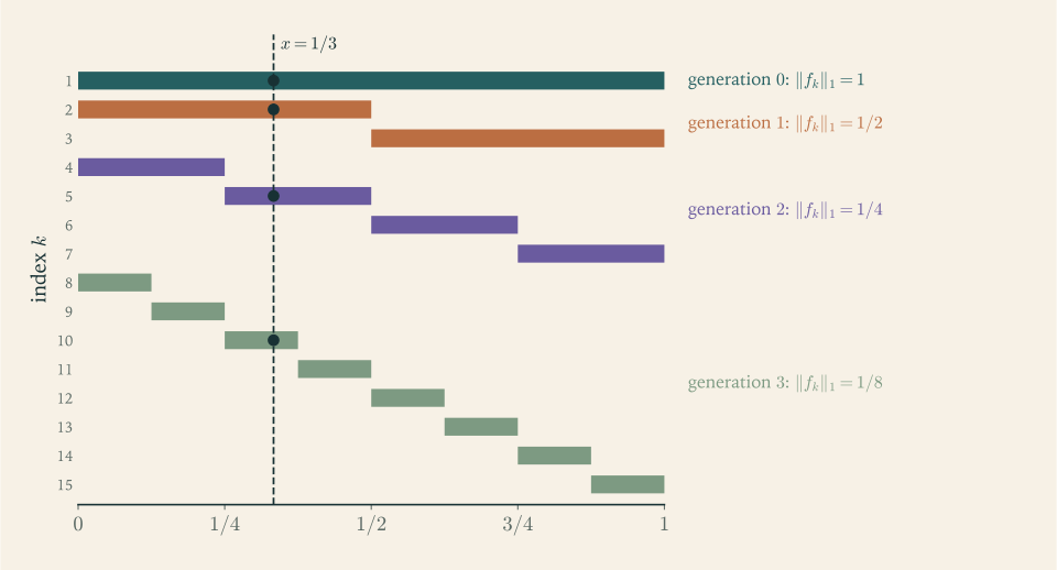
So \(f_1\) is the indicator of \([0,1]\) ; \(f_2,f_3\) are the indicators of the two halves; \(f_4,\dots,f_7\) of the four quarters; and so on. Within each generation the interval moves from left to right like the carriage of a typewriter, and then returns with half the width.
Convergence in norm and in measure. For \(2^m\le k<2^{m+1}\) , \(\lVert f_k\rVert_p=2^{-m/p}\) for every finite \(p\) , and \(\lambda(\{f_k>\varepsilon\})=2^{-m}\) for \(0<\varepsilon<1\) . Both tend to \(0\) as \(k\to\infty\) . So \(f_k\to0\) in every \(L^p\) , \(p<\infty\) , and in measure.
No pointwise convergence anywhere. Fix \(x\in[0,1]\) . In every generation \(m\) the dyadic intervals of length \(2^{-m}\) cover \([0,1]\) , so at least one \(f_k\) with \(2^m\le k<2^{m+1}\) equals \(1\) at \(x\) ; and for \(m\ge2\) at least one equals \(0\) there, since the closed intervals of a generation containing \(x\) number at most two. (For \(m=1\) the point \(x=\tfrac12\) lies in both halves.) Hence the sequence \(f_k(x)\) takes the values \(0\) and \(1\) infinitely often and converges for no \(x\) at all. For \(x=\tfrac13\) , the indices \(k\le31\) with \(f_k(x)=1\) are exactly \(k=1,2,5,10,21\) , one in each generation.
The subsequence. Corollary 8.3 promises a subsequence converging a.e. Here \(f_{2^m}=\mathbf 1_{[0,2^{-m}]}\) will do: it tends to \(0\) at every \(x>0\) .
Figure 8.1 shows the first four generations and the points at which the vertical line \(x=\tfrac13\) is hit.
Example 8.3: Four sequences, four patterns of convergence
Let \(s_n=n\mathbf 1_{(0,1/n)}\) be the spike, \(b_n=\mathbf 1_{[n,n+1]}\) the sliding block, \(w_n=\tfrac1n\mathbf 1_{[0,n]}\) the flattening block, and \(f_k\) the typewriter sequence. The candidate limit is \(0\) in each case. Their norms are
and the measures of the sets where they exceed a small \(\varepsilon\) are \(\tfrac1n\) , \(1\) , eventually \(0\) , and \(2^{-m}\) .
| Sequence | Almost everywhere | In measure | In \(L^1\) | In \(L^2\) |
|---|---|---|---|---|
| Spike \(s_n\) | yes | yes | no | no |
| Sliding block \(b_n\) | yes | no | no | no |
| Flattening block \(w_n\) | yes | yes | no | yes |
| Typewriter \(f_k\) | no | yes | yes | yes |
The sliding block shows that Proposition 8.5(c) needs finite measure. The spike shows that convergence a.e. and in measure together do not give convergence in any \(L^p\) . The flattening block converges in \(L^2\) , since \(\lVert w_n\rVert_2=n^{-1/2}\) , but not in \(L^1\) , where \(\lVert w_n\rVert_1=1\) : convergence in one \(L^p\) says nothing about another on a space of infinite measure. And the typewriter shows that convergence in norm does not give convergence at even one point.
Common mistake. Passing from “\(f_n\to f\) in \(L^p\) ” to “\(f_n(x)\to f(x)\) for almost every \(x\) ”. Only a subsequence is guaranteed to converge a.e. When an argument needs pointwise convergence, extract the subsequence explicitly and check that the conclusion, once proved for it, transfers to the whole sequence.
8.3 Dense classes of functions
An element of \(L^p\) is an abstract object. To prove something about all of them one usually proves it first for a convenient class and then extends by approximation. For this the class must be dense: every element of \(L^p\) must be a limit, in norm, of members of the class.
Theorem 8.6 (density of simple functions). Let \(1\le p<\infty\) . The simple functions that vanish outside a set of finite measure are dense in \(L^p(\mu)\) .
Proof. Let \(f\in L^p\) . By Corollary 3.10 there are simple functions \(\psi_n\to f\) pointwise with \(\lvert\psi_n\rvert\le\lvert f\rvert\) . Each \(\psi_n\) is in \(L^p\) , so each set on which it takes a nonzero value has finite measure. Moreover \(\lvert\psi_n-f\rvert^p\le2^p\lvert f\rvert^p\) , which is integrable, so \(\lVert\psi_n-f\rVert_p\to0\) by dominated convergence.
On the line the approximating functions can be made much more concrete. A step function is a finite linear combination of indicators of bounded intervals, and \(C_c(\mathbb R)\) denotes the continuous functions that vanish outside some bounded interval.
Theorem 8.7 (density of step functions and of continuous functions). Let \(1\le p<\infty\) . The step functions are dense in \(L^p(\mathbb R)\) , and so is \(C_c(\mathbb R)\) .
Proof. By Theorem 8.6 and the triangle inequality it is enough to approximate \(\mathbf 1_E\) for a measurable set \(E\) with \(\lambda(E)<\infty\) . Given \(\varepsilon>0\) , Corollary 2.11 provides a finite union \(J\) of bounded intervals with \(\lambda(E\triangle J)<\varepsilon^p\) . Then \(\mathbf 1_J\) is a step function and
So step functions are dense. For continuous functions it now suffices to approximate the indicator of one bounded interval \([a,b]\) . For \(\delta>0\) let \(h_\delta\) be the trapezoidal function equal to \(1\) on \([a,b]\) , to \(0\) outside \((a-\delta,b+\delta)\) , and linear on the two remaining intervals. It is continuous with bounded support, it differs from \(\mathbf 1_{[a,b]}\) by at most \(1\) and only on a set of measure \(2\delta\) , so \(\lVert h_\delta-\mathbf 1_{[a,b]}\rVert_p\le(2\delta)^{1/p}\to0\) .
The proof is a chain of three approximations, each resting on an earlier chapter: an \(L^p\) function by a simple function (Chapter 3), a measurable set by a finite union of intervals (Chapter 2), and an interval by a trapezoid. The same statements hold on \(\mathbb R^d\) with rectangles in place of intervals.
Example 8.4: Continuous functions are not dense for the supremum norm
In \(L^\infty(0,1)\) let \(f=\mathbf 1_{(0,1/2]}\) , and let \(g\) be any continuous function on \([0,1]\) . Suppose \(\lVert f-g\rVert_\infty=c<\tfrac12\) . Then \(g\ge1-c\) almost everywhere on \((0,\tfrac12]\) . A set of full measure in an interval is dense in it, so by continuity \(g\ge1-c\) on all of \([0,\tfrac12]\) ; in particular \(g(\tfrac12)\ge1-c>\tfrac12\) . In the same way \(g\le c\) almost everywhere on \((\tfrac12,1)\) , hence on \([\tfrac12,1]\) , so \(g(\tfrac12)\le c<\tfrac12\) . The contradiction shows
with equality for the constant \(g=\tfrac12\) . A jump cannot be approximated uniformly by continuous functions, even after discarding null sets. Theorem 8.7 fails for \(p=\infty\) , and the proof shows where: the trapezoid differs from the indicator on a set of small measure, which is small in \(L^p\) for finite \(p\) and not small at all in \(L^\infty\) .
Example 8.5: Approximating a ramp by step functions
Let \(f(x)=x\) on \([0,1]\) and let \(s_n\) be the step function equal on each interval \([\tfrac{i-1}n,\tfrac in)\) to the value of \(f\) at its midpoint, \(\tfrac{2i-1}{2n}\) . On each such interval \(f-s_n\) runs linearly from \(-\tfrac1{2n}\) to \(\tfrac1{2n}\) , so
With \(n=10\) the error is about \(0.0289\) . Here density is explicit and comes with a rate; for a general element of \(L^2\) Theorem 8.7 guarantees approximants and gives no rate at all.
Density arguments have a standard shape, shown in the next proof: establish the statement for the dense class by direct computation, and then show that the set of functions for which it holds is closed under limits in norm.
Corollary 8.8 (continuity of translation). For \(h\in\mathbb R\) let \((\tau_hf)(x)=f(x-h)\) . If \(1\le p<\infty\) and \(f\in L^p(\mathbb R)\) , then \(\lVert\tau_hf-f\rVert_p\to0\) as \(h\to0\) .
Proof. Let \(\varepsilon>0\)
and choose \(g\in C_c(\mathbb R)\)
with \(\lVert f-g\rVert_p<\varepsilon\)
, vanishing outside \([-R,R]\)
. A continuous function with bounded support is uniformly continuous (math.real-analysis.heine-cantor), so \(\sup_x\lvert g(x-h)-g(x)\rvert\to0\)
as \(h\to0\)
; for \(\lvert h\rvert\le1\)
the function \(\tau_hg-g\)
vanishes outside \([-R-1,R+1]\)
, and therefore
Lebesgue measure is translation invariant, so \(\lVert\tau_h(f-g)\rVert_p=\lVert f-g\rVert_p<\varepsilon\) . By the triangle inequality,
for all sufficiently small \(h\) .
Example 8.6: Translating an indicator
Let \(f=\mathbf 1_{[0,1]}\) and \(0<h\le1\) . Then \(\tau_hf=\mathbf 1_{[h,1+h]}\) , and \(\lvert\tau_hf-f\rvert\) is the indicator of \([0,h)\cup(1,1+h]\) , a set of measure \(2h\) . Hence
For finite \(p\) this tends to \(0\) with \(h\) , as Corollary 8.8 says, though slowly when \(p\) is large: for \(h=0.01\) it is \(0.02\) in \(L^1\) and about \(0.1414\) in \(L^2\) . In \(L^\infty\) it does not tend to \(0\) at all. Translation is continuous on \(L^p\) exactly in the range of exponents where continuous functions are dense.
Density also explains how close a measurable function is to a continuous one, completing the picture begun by Egorov’s theorem.
Theorem 8.9 (Lusin). Let \(f:[a,b]\to\mathbb R\) be Lebesgue measurable. For every \(\varepsilon>0\) there is a compact set \(K\subseteq[a,b]\) with \(\lambda([a,b]\setminus K)<\varepsilon\) such that the restriction of \(f\) to \(K\) is continuous.
Proof. Suppose first that \(f\)
is bounded, so that \(f\in L^1([a,b])\)
. By Theorem 8.7 there are continuous functions \(g_n\)
with \(\lVert g_n-f\rVert_1\to0\)
, and by Corollary 8.3 a subsequence converges to \(f\)
a.e. on \([a,b]\)
. By Egorov’s theorem there is a measurable \(E\subseteq[a,b]\)
with \(\lambda([a,b]\setminus E)<\varepsilon/2\)
on which the subsequence converges to \(f\)
uniformly. By Theorem 2.10 there is a compact \(K\subseteq E\)
with \(\lambda(E\setminus K)<\varepsilon/2\)
. On \(K\)
the function \(f\)
is a uniform limit of continuous functions, hence continuous (math.real-analysis.uniform-limit-continuity).
For a general measurable \(f\) , apply this to the bounded measurable function \(\arctan f\) to obtain \(K\) . Then \(f=\tan(\arctan f)\) is continuous on \(K\) , because \(\tan\) is continuous on \((-\tfrac\pi2,\tfrac\pi2)\) .
The conclusion is about the restriction of \(f\) to \(K\) , not about continuity of \(f\) at the points of \(K\) . The indicator of the rationals is discontinuous at every point of \([0,1]\) , yet its restriction to any compact set of irrationals is the constant \(0\) .
The spaces \(L^p\) are complete, and their elements can be approximated by simple, step, and continuous functions. Chapter 4 showed that every nonnegative measurable function \(f\) defines a measure \(E\mapsto\int_Ef\,d\mu\) . Which measures arise in that way?
Exercises
-
For the flattening block \(w_n=\tfrac1n\mathbf 1_{[0,n]}\) on \(\mathbb R\) compute \(\lVert w_n\rVert_p\) for \(1\le p\le\infty\) and decide, for each \(p\) , whether \(w_n\to0\) in \(L^p\) .
Answer
For \(p<\infty\) , \(\lVert w_n\rVert_p=(n^{-p}\cdot n)^{1/p}=n^{1/p-1}\) , and \(\lVert w_n\rVert_\infty=\tfrac1n\) . So \(w_n\to0\) in \(L^p\) for every \(p\in(1,\infty]\) , and not for \(p=1\) , where the norm is \(1\) for all \(n\) .
-
Write out the proof that \(L^\infty(\mu)\) is complete, stating exactly which null sets are discarded and why their union is null.
Solution
Let \((f_n)\) be a Cauchy sequence in \(L^\infty(\mu)\) ; fix one representative of each class.
The null sets. For each pair \((m,n)\) let \(N_{m,n}=\{x:\lvert f_m(x)-f_n(x)\rvert>\lVert f_m-f_n\rVert_\infty\}\) . By the remark after Definition 7.2 the essential supremum is attained, so each \(N_{m,n}\) is null. There are countably many pairs, and a countable union of null sets is null by countable subadditivity; let \(N=\bigcup_{m,n}N_{m,n}\) .
The pointwise limit. For \(x\notin N\) and all \(m,n\) , \(\lvert f_m(x)-f_n(x)\rvert\le\lVert f_m-f_n\rVert_\infty\) . The right side is small for large \(m,n\) , so \((f_n(x))\) is a Cauchy sequence of real numbers and has a limit \(f(x)\) . Put \(f=0\) on \(N\) . Then \(f=\lim_nf_n\mathbf 1_{N^c}\) is measurable.
Convergence in norm. Given \(\varepsilon>0\) choose \(n_0\) with \(\lVert f_m-f_n\rVert_\infty<\varepsilon\) for \(m,n\ge n_0\) . For \(x\notin N\) and \(n\ge n_0\) , letting \(m\to\infty\) in \(\lvert f_m(x)-f_n(x)\rvert<\varepsilon\) gives \(\lvert f(x)-f_n(x)\rvert\le\varepsilon\) . So \(\lvert f-f_n\rvert\le\varepsilon\) off the null set \(N\) , that is, \(\lVert f-f_n\rVert_\infty\le\varepsilon\) for \(n\ge n_0\) . In particular \(\lVert f\rVert_\infty\le\lVert f_{n_0}\rVert_\infty+\varepsilon<\infty\) , so \(f\in L^\infty\) . The point of collecting all the exceptional sets into one null set at the start is that afterwards the argument is simply uniform convergence on \(N^c\) .
-
Let \(f_n\in L^1(\mu)\) with \(\lVert f_{n+1}-f_n\rVert_1\le2^{-n}\) for all \(n\) . Prove that \(f_n\) converges almost everywhere and in \(L^1\) , and explain why the typewriter sequence does not contradict this.
Solution
Put \(g_n=f_{n+1}-f_n\) . Then \(\sum_n\lVert g_n\rVert_1\le\sum_n2^{-n}<\infty\) , so Lemma 8.1 with \(p=1\) applies: the series \(\sum_ng_n\) converges absolutely a.e. and in \(L^1\) . Its partial sums are \(\sum_{n<N}g_n=f_N-f_1\) . Hence \(f_N\) converges a.e., and in \(L^1\) , to \(f=f_1+\sum_ng_n\in L^1\) . This is the first half of the proof of Theorem 8.2 with the subsequence already given.
The typewriter sequence converges to \(0\) in \(L^1\) and at no point, and it is Cauchy in \(L^1\) . There is no contradiction, because it is not rapidly Cauchy: within generation \(m\) consecutive terms are indicators of adjacent intervals of length \(2^{-m}\) , so \(\lVert f_{k+1}-f_k\rVert_1=2\cdot2^{-m}\) for each of the \(2^m-1\) consecutive pairs in that generation, and those differences alone sum to \(2-2^{1-m}\) . Summing over generations, \(\sum_k\lVert f_{k+1}-f_k\rVert_1=\infty\) . A Cauchy sequence need not have summable increments; it always has a subsequence that does, and the subsequence \(f_{2^m}\) is one.
-
For the typewriter sequence of Example 8.2 and the point \(x=\tfrac15\) , list the indices \(k\le63\) with \(f_k(x)=1\) .
Answer
\(k=1,2,4,9,19,38\) . In generation \(m\) the point \(\tfrac15\) lies in the dyadic interval with \(j=\lfloor2^m/5\rfloor\) , giving \(j=0,0,0,1,3,6\) for \(m=0,\dots,5\) and \(k=2^m+j\) .
-
Prove that limits in measure are unique up to null sets: if \(f_n\to f\) and \(f_n\to g\) in measure, then \(f=g\) almost everywhere.
Hint
For \(\varepsilon>0\) , \(\{\lvert f-g\rvert>2\varepsilon\}\subseteq\{\lvert f-f_n\rvert>\varepsilon\}\cup\{\lvert f_n-g\rvert>\varepsilon\}\) for every \(n\) . Let \(n\to\infty\) to get \(\mu(\{\lvert f-g\rvert>2\varepsilon\})=0\) , then take the union over \(\varepsilon=\tfrac1m\) .
-
Let \(1\le p<\infty\) , let \(f_n\to f\) in measure, and suppose \(\lvert f_n\rvert\le g\) for all \(n\) with \(g\in L^p\) . Prove that \(f_n\to f\) in \(L^p\) .
Solution
Suppose, for contradiction, that \(\lVert f_n-f\rVert_p\) does not tend to \(0\) . Then there are \(\delta>0\) and a subsequence \((f_{n_j})\) with \(\lVert f_{n_j}-f\rVert_p\ge\delta\) for all \(j\) . This subsequence still converges to \(f\) in measure, so by Proposition 8.5(b) it has a further subsequence \((f_{n_{j_i}})\) converging to \(f\) almost everywhere.
Along that sub-subsequence, \(\lvert f_{n_{j_i}}\rvert\le g\) , and passing to the limit, \(\lvert f\rvert\le g\) a.e. Hence
\[ \lvert f_{n_{j_i}}-f\rvert^p\le(2g)^p, \]which is integrable because \(g\in L^p\) , and the left side tends to \(0\) a.e. By dominated convergence \(\lVert f_{n_{j_i}}-f\rVert_p\to0\) , contradicting \(\lVert f_{n_j}-f\rVert_p\ge\delta\) .
The pattern is worth isolating. Dominated convergence needs convergence almost everywhere, which convergence in measure supplies only along subsequences. But a sequence of real numbers tends to \(0\) as soon as every subsequence has a further subsequence tending to \(0\) , and that principle transfers the theorem from subsequences to the whole sequence. So the dominated convergence theorem remains true with “in measure” in place of “almost everywhere”.
-
A student argues: “\(f_n\to f\) in \(L^1\) , so \(f_n(x)\to f(x)\) for almost every \(x\) , so by Fatou’s lemma \(\int\lvert f\rvert\le\liminf\int\lvert f_n\rvert\) .” The conclusion is true. Identify the false step and repair the argument.
Answer
The false step is “so \(f_n(x)\to f(x)\) for almost every \(x\) ”; the typewriter sequence converges in \(L^1\) and nowhere pointwise. Repair: choose a subsequence along which \(\int\lvert f_{n}\rvert\) tends to \(\liminf_n\int\lvert f_n\rvert\) , then by Corollary 8.3 a further subsequence converging to \(f\) a.e., and apply Fatou’s lemma to that. (Here the conclusion also follows at once from \(\lvert\lVert f_n\rVert_1-\lVert f\rVert_1\rvert\le\lVert f_n-f\rVert_1\) , with equality of the limits.)
-
Among the functions that are constant on \([0,\tfrac12)\) and on \([\tfrac12,1]\) , find the one closest to \(x^2\) in \(L^2(0,1)\) , and compute the distance.
Solution
Let \(s=c_1\mathbf 1_{[0,1/2)}+c_2\mathbf 1_{[1/2,1]}\) . Then
\[ \lVert x^2-s\rVert_2^2=\int_0^{1/2}(x^2-c_1)^2\,dx+\int_{1/2}^1(x^2-c_2)^2\,dx, \]and the two constants can be chosen independently. For an interval \(I\) of length \(\ell\) , the quadratic \(c\mapsto\int_I(x^2-c)^2\,dx\) is minimized where its derivative \(-2\int_I(x^2-c)\,dx\) vanishes, that is, at the average \(c=\frac1\ell\int_Ix^2\,dx\) . So
\[ c_1=2\int_0^{1/2}x^2\,dx=\frac1{12},\qquad c_2=2\int_{1/2}^1x^2\,dx=2\Bigl(\frac13-\frac1{24}\Bigr)=\frac7{12}. \]At the minimizer, \(\int_I(x^2-c)^2=\int_Ix^4-\ell c^2\) , so
\[ \lVert x^2-s\rVert_2^2=\int_0^1x^4\,dx-\frac12\Bigl(\frac1{144}+\frac{49}{144}\Bigr)=\frac15-\frac{25}{144}=\frac{19}{720}, \]and the distance is \(\sqrt{19/720}\approx0.1624\) . The best step function takes on each piece the mean value of the target there. This is the orthogonal projection of \(x^2\) onto the two-dimensional space of such step functions, a fact about \(L^2\) that the other \(L^p\) spaces do not share.
-
Show that \(C_c(\mathbb R)\) is not dense in \(L^\infty(\mathbb R)\) by exhibiting a bounded function whose distance from every element of \(C_c(\mathbb R)\) is at least \(1\) .
Hint
Take the constant function \(1\) . Any \(g\in C_c(\mathbb R)\) vanishes outside a bounded interval, and the complement of that interval has positive measure, so \(\lvert1-g\rvert=1\) on a set of positive measure.
-
For \(f(x)=e^{-\lvert x\rvert}\) on \(\mathbb R\) and \(h>0\) compute \(\lVert\tau_hf-f\rVert_1\) in closed form, and verify its limits as \(h\to0\) and as \(h\to\infty\) .
Solution
For \(h>0\) the function \(\tau_hf(x)=e^{-\lvert x-h\rvert}\) is the reflection of \(f\) in the point \(x=\tfrac h2\) , so \(\lvert\tau_hf-f\rvert\) is symmetric about \(\tfrac h2\) , and \(\tau_hf\ge f\) exactly for \(x\ge\tfrac h2\) . Hence
\[ \lVert\tau_hf-f\rVert_1=2\int_{h/2}^\infty\bigl(e^{-\lvert x-h\rvert}-e^{-x}\bigr)\,dx . \]Compute the two pieces. First, \(\int_{h/2}^\infty e^{-x}\,dx=e^{-h/2}\) . Second,
\[ \int_{h/2}^\infty e^{-\lvert x-h\rvert}\,dx=\int_{h/2}^he^{x-h}\,dx+\int_h^\infty e^{-(x-h)}\,dx=(1-e^{-h/2})+1 . \]Therefore
\[ \lVert\tau_hf-f\rVert_1=2\bigl(2-e^{-h/2}-e^{-h/2}\bigr)=4\bigl(1-e^{-h/2}\bigr). \]As \(h\to0\) this behaves like \(2h\) and tends to \(0\) , as Corollary 8.8 requires. As \(h\to\infty\) it tends to \(4=2\lVert f\rVert_1\) : the two copies of \(f\) become effectively disjoint, and the norm of the difference is the sum of the norms. For example, at \(h=1\) the value is \(4(1-e^{-1/2})\approx1.5739\) .
-
Let \(f\in L^1(\mathbb R)\) . Prove that \(\int_{\mathbb R}f(x)\cos(tx)\,dx\to0\) as \(t\to\infty\) , by treating indicators of intervals first and then using Theorem 8.7.
Solution
Indicators. For a bounded interval with endpoints \(a<b\) and \(t>0\) ,
\[ \Bigl\lvert\int_a^b\cos(tx)\,dx\Bigr\rvert=\Bigl\lvert\frac{\sin(tb)-\sin(ta)}{t}\Bigr\rvert\le\frac2t\longrightarrow0 . \]Step functions. A step function \(s\) is a finite linear combination of such indicators, so \(\int s(x)\cos(tx)\,dx\to0\) by linearity.
General \(f\) . Let \(\varepsilon>0\) . By Theorem 8.7 there is a step function \(s\) with \(\lVert f-s\rVert_1<\varepsilon\) . Since \(\lvert\cos\rvert\le1\) ,
\[ \Bigl\lvert\int f(x)\cos(tx)\,dx\Bigr\rvert\le\int\lvert f-s\rvert\,dx+\Bigl\lvert\int s(x)\cos(tx)\,dx\Bigr\rvert<\varepsilon+\Bigl\lvert\int s(x)\cos(tx)\,dx\Bigr\rvert . \]The last term is less than \(\varepsilon\) for all large \(t\) . Hence the upper limit of the left side is at most \(2\varepsilon\) , for every \(\varepsilon\) .
This is the Riemann–Lebesgue lemma, and the proof is the density method in its purest form: an explicit computation on the simplest functions, and one inequality, uniform in \(t\) , that lets the statement pass to limits in \(L^1\) . Dominated convergence would not have worked here, because \(f(x)\cos(tx)\) does not converge pointwise as \(t\to\infty\) .
-
Prove that for \(1\le p<\infty\) the step functions with rational values and rational endpoints form a countable dense subset of \(L^p(\mathbb R)\) , and that \(L^\infty(\mathbb R)\) has no countable dense subset.
Hint
Rational step functions form a countable set; approximate real coefficients and endpoints by rational ones and use Theorem 8.7. For \(L^\infty\) , the functions \(\mathbf 1_{[0,t]}\) , \(t>0\) , are uncountably many and pairwise at distance \(1\) ; a dense set must contain a point within \(\tfrac12\) of each, and these points are distinct.
-
Suppose \(f_n\to f\) in \(L^p\) and \(f_n\to g\) almost everywhere. Prove that \(f=g\) almost everywhere.
Answer
By Corollary 8.3 a subsequence \(f_{n_k}\to f\) a.e. The same subsequence converges to \(g\) a.e. Limits of real sequences are unique, so \(f=g\) outside the union of two null sets.
-
Use Theorem 8.9 to prove that every Lebesgue measurable \(f:[a,b]\to\mathbb R\) is the almost-everywhere limit of a sequence of continuous functions.
Hint
For each \(n\) take compact \(K_n\) with \(\lambda([a,b]\setminus K_n)<2^{-n}\) and \(f\) continuous on \(K_n\) ; extend \(f\) from \(K_n\) to a continuous \(g_n\) on \([a,b]\) by linear interpolation across the gaps. Then \(g_n=f\) on \(K_n\) , and by Proposition 1.12 almost every \(x\) lies in \(K_n\) for all large \(n\) .
-
Let \(f_n\) be the continuous function on \([0,1]\) that is \(0\) on \([0,\tfrac12]\) , \(1\) on \([\tfrac12+\tfrac1n,1]\) , and linear between. Compute \(\lVert f_n-\mathbf 1_{(1/2,1]}\rVert_1\) and conclude that the continuous functions with the \(L^1\) norm are not complete.
Solution
The difference \(\mathbf 1_{(1/2,1]}-f_n\) vanishes outside \((\tfrac12,\tfrac12+\tfrac1n)\) , and on that interval it decreases linearly from \(1\) to \(0\) . Its graph is a triangle with base \(\tfrac1n\) and height \(1\) , so
\[ \lVert f_n-\mathbf 1_{(1/2,1]}\rVert_1=\frac1{2n}\longrightarrow0 . \]Hence \((f_n)\) converges in \(L^1(0,1)\) , so it is a Cauchy sequence there, and each \(f_n\) is continuous. Suppose some continuous \(g\) on \([0,1]\) had \(\lVert f_n-g\rVert_1\to0\) . Limits in \(L^1\) are unique, so \(g=\mathbf 1_{(1/2,1]}\) almost everywhere. Then \(g=0\) a.e. on \([0,\tfrac12]\) and \(g=1\) a.e. on \((\tfrac12,1]\) ; by continuity \(g=0\) on all of \([0,\tfrac12]\) and \(g=1\) on all of \([\tfrac12,1]\) , which is impossible at the point \(\tfrac12\) .
So the space of continuous functions on \([0,1]\) with the norm \(\lVert\cdot\rVert_1\) contains a Cauchy sequence with no limit in the space: it is not complete. By Theorem 8.7 it is dense in \(L^1(0,1)\) , and by Theorem 8.2 that space is complete. In this precise sense \(L^1\) is to the continuous functions what \(\mathbb R\) is to \(\mathbb Q\) .
-
Let \(\mu(X)<\infty\) . Prove that \(f_n\to f\) in measure if and only if every subsequence of \((f_n)\) has a further subsequence converging to \(f\) almost everywhere.
Hint
One direction is Proposition 8.5(b) applied to subsequences. For the other, argue by contradiction as in Exercise 8.6: if \(\mu(\{\lvert f_n-f\rvert>\varepsilon\})\) does not tend to \(0\) , extract a subsequence along which it stays above some \(\delta\) , then a further subsequence converging a.e., and apply Proposition 8.5(c).
-
Let \(1<p<\infty\) with conjugate \(q\) , \(f\in L^p(\mathbb R)\) , and \(g\in L^q(\mathbb R)\) , both Borel. Prove that \(f*g\) is defined everywhere, bounded by \(\lVert f\rVert_p\lVert g\rVert_q\) , and uniformly continuous.
Solution
Defined and bounded. Fix \(x\) . The function \(y\mapsto f(x-y)\) is Borel, and by invariance of Lebesgue measure under translation and reflection its \(L^p\) norm is \(\lVert f\rVert_p\) . By Hölder’s inequality \(y\mapsto f(x-y)g(y)\) is integrable, with
\[ \lvert(f*g)(x)\rvert\le\int\lvert f(x-y)\rvert\,\lvert g(y)\rvert\,dy\le\lVert f\rVert_p\,\lVert g\rVert_q . \]So \(f*g\) is defined at every point, not merely almost everywhere, and is bounded.
Uniformly continuous. Let \(\tilde f(u)=f(-u)\) , so that \(f(x-y)=\tilde f(y-x)=(\tau_x\tilde f)(y)\) . For any \(x\) and \(h\) , Hölder’s inequality gives
\[ \lvert(f*g)(x+h)-(f*g)(x)\rvert\le\int\lvert\tau_{x+h}\tilde f-\tau_x\tilde f\rvert\,\lvert g\rvert\,dy\le\lVert\tau_{x+h}\tilde f-\tau_x\tilde f\rVert_p\,\lVert g\rVert_q=\lVert\tau_h\tilde f-\tilde f\rVert_p\,\lVert g\rVert_q, \]the last step by translation invariance. The right side does not depend on \(x\) , and it tends to \(0\) as \(h\to0\) by Corollary 8.8, since \(\tilde f\in L^p\) with \(p<\infty\) . That is uniform continuity. The hypothesis \(p<\infty\) was used only here; if \(p=\infty\) and \(q=1\) , apply the same argument with the roles of \(f\) and \(g\) exchanged.