Chapter 1 ended with a vehicle that cannot exist: a single kerosene stage asked for \(9.4\ \mathrm{km/s}\) comes out with a negative payload. Yet kerosene rockets reach orbit routinely, and the Falcon 9 whose figures were used there delivers about 4 percent of its liftoff mass. The difference is that it is two rockets, one riding on the other. The lower one burns out at a few kilometres per second and is thrown away; the upper one starts from that speed with its own tanks full.
That raises three questions, which organize this chapter. Why does cutting a vehicle in two change the arithmetic at all, when the rocket equation said only the mass ratio matters? Where should the cut be made: how much of the velocity should each stage supply? And once a vehicle is laid out, what does a kilogram of extra structure, or a second of extra specific impulse, cost or buy? The second question is a constrained optimization problem of exactly the kind a Lagrange multiplier solves, and the multiplier turns out to answer part of the third. The chapter ends with the first numerical design of the reference launcher.
2.1 Three kinds of mass
The rocket equation needs only two masses, initial and final. A designer needs to know what the final mass is made of, because only part of it is useful. Split the mass of a rocket stage and its cargo three ways.
Propellant, \(m_p\) , is what the stage burns. Structure, \(m_s\) , is everything else that belongs to the stage: tanks, engines, pumps, the frame that carries the thrust, wiring, and any propellant left unburned. Payload, \(m_L\) , is whatever the stage carries that is not part of it. For the top stage that is the satellite. For a lower stage it is everything stacked above it, upper stages included, since from the lower stage’s point of view an upper stage is cargo.
At ignition the mass is \(m_0=m_s+m_p+m_L\) , and at burnout it is \(m_f=m_s+m_L\) . Three ratios describe the split.
Definition 2.1 (structural coefficient, payload ratio, payload fraction). For a stage with structure \(m_s\) and propellant \(m_p\) carrying payload \(m_L\) :
The structural coefficient \(\varepsilon\) is the fraction of the stage’s own mass that is not propellant. The payload ratio \(\lambda\) compares the cargo with the stage that carries it. The payload fraction \(\pi\) compares the cargo with the whole stack.
The structural coefficient is defined without the payload on purpose. It is a property of the hardware, a measure of how lightly the stage is built, and it stays the same whatever the stage is asked to carry. The other two depend on the cargo. Typical values come from real stages: using the masses quoted in Chapter 1, the Falcon 9 first stage has \(\varepsilon=22\,200/433\,100=0.051\) and the Saturn V’s hydrogen second stage \(\varepsilon=36\,150/479\,900=0.075\) (secondary compilation; see sources). Across the two Falcon 9 stages and three Saturn V stages for which that compilation gives masses, the coefficient runs from about \(0.04\) to \(0.13\) ; why stages cannot be made much lighter is a subject for Chapter 6.
Proposition 2.1 (mass ratio and payload fraction of a stage). With the notation of Definition 2.1 and \(\mathcal R=m_0/m_f\) ,
The mass ratio satisfies \(1<\mathcal R\le1/\varepsilon\) , with equality on the right only when the payload is zero. If the stage delivers an ideal velocity increment \(\Delta v=c\ln\mathcal R\) , its payload fraction is
which is positive only for \(\Delta v<c\,\ln(1/\varepsilon)\) .
Proof. Divide \(m_0=m_s+m_p+m_L\) and \(m_f=m_s+m_L\) by \(m_s+m_p\) to get \(m_0/(m_s+m_p)=1+\lambda\) and \(m_f/(m_s+m_p)=\varepsilon+\lambda\) ; their quotient is \(\mathcal R\) , and \(\pi=m_L/m_0=\lambda/(1+\lambda)\) . Solving \(\mathcal R(\varepsilon+\lambda)=1+\lambda\) for \(\lambda\) gives \(\lambda=(1-\varepsilon\mathcal R)/(\mathcal R-1)\) , and substituting into \(\lambda/(1+\lambda)\) gives the second form of \(\pi\) . Since \(\lambda\ge0\) , the numerator \(1-\varepsilon\mathcal R\) is nonnegative, so \(\mathcal R\le1/\varepsilon\) . Finally put \(\mathcal R=e^{\Delta v/c}\) and divide numerator and denominator by \(\mathcal R\) .
The bound \(\mathcal R\le1/\varepsilon\) is the algebraic form of the last section of Chapter 1. Even with no payload, a stage cannot have a mass ratio larger than the reciprocal of its structural coefficient, so the most velocity it can supply is \(c\ln(1/\varepsilon)\) . A stage with \(\varepsilon=0.06\) tops out at \(\mathcal R=16.7\) . This is a statement about one stage. It says nothing yet about a vehicle made of several.
A warning about conventions. Some texts divide the structure by the stage’s initial mass including payload, \(m_s/m_0\) , and call that the structural fraction (MIT 16.50 notes; see sources). That number changes when the payload changes. Exercise 3 relates the two conventions. When you read a structural figure in another source, find out which mass is in its denominator.
Example 2.1: What one stage can and cannot do
Question. A kerosene stage has structural coefficient \(\varepsilon=0.06\) (illustrative) and effective exhaust velocity \(c=3049.9\ \mathrm{m/s}\) , the vacuum value for \(I_{sp}=311\ \mathrm s\) used in Chapter 1. What payload fraction does it achieve for \(\Delta v=4.7\ \mathrm{km/s}\) and for \(\Delta v=9.4\ \mathrm{km/s}\) , and what is the largest \(\Delta v\) it can supply?
Half the orbital requirement. \(e^{-4700/3049.9}=e^{-1.5411}=0.2142\) , so
A sixth of the stack is payload.
The full requirement. \(e^{-9400/3049.9}=0.04586\) , so
Negative: the stage cannot do it, in agreement with Example 1.3.
The limit. With zero payload, \(\Delta v_{\max}=c\ln(1/\varepsilon)=(3049.9\ \mathrm{m/s})\ln(16.67)=(3049.9)(2.8134)=8581\ \mathrm{m/s}\) .
Check. The payload fraction must fall to zero exactly at the limit: \(e^{-8581/3049.9}=0.0600=\varepsilon\) . And doubling \(\Delta v\) did far worse than halving the payload: from \(16.4\) percent to less than nothing. That is the exponential at work, and it suggests the remedy. Two stages that each supply \(4.7\ \mathrm{km/s}\) would each carry a sixth of their stack, for an overall payload of about \(1/36\) of liftoff mass.
2.2 Stacking stages
In serial staging the stages fire one after another. Number them in firing order, \(k=1,\dots,N\) . The bookkeeping uses one symbol with one meaning: \(m_{0,k}\) is the mass of the whole stack at the moment stage \(k\) ignites, that is, stage \(k\) , every stage above it, and the final payload. The payload of stage \(k\) is then the stack above it, \(m_{0,k+1}\) , and by convention \(m_{0,N+1}=m_L\) , the payload delivered to orbit.
Follow the mass through one stage’s operation:
During the burn the rocket equation applies with mass ratio \(\mathcal R_k=m_{0,k}/m_{f,k}\) . At separation the mass drops by \(m_{s,k}\) with no change in velocity: the empty stage is released, not thrown, so it carries away no momentum relative to the vehicle and Proposition 1.1 gives no velocity change. The next stage ignites at the speed the previous one reached.
Proposition 2.2 (velocity and payload of a staged vehicle). For \(N\) serial stages with effective exhaust velocities \(c_k\) and mass ratios \(\mathcal R_k\) , with no external forces during the burns, the total ideal velocity increment and the overall payload fraction \(\pi_L=m_L/m_{0,1}\) are
Proof. Each burn contributes \(c_k\ln\mathcal R_k\) by Proposition 1.2, separations contribute nothing, and velocity changes add. The product telescopes: \(\pi_1\pi_2\cdots\pi_N=(m_{0,2}/m_{0,1})(m_{0,3}/m_{0,2})\cdots(m_L/m_{0,N})=m_L/m_{0,1}\) . The expression for \(\pi_k\) is Proposition 2.1 applied to stage \(k\) with payload \(m_{0,k+1}\) .
Velocities add and payload fractions multiply. The whole of staging design is the tension between those two operations.
Common mistake. Treating the product \(\mathcal R_1\mathcal R_2\) as the mass ratio of the vehicle and writing \(\Delta v=\bar c\,\ln(\mathcal R_1\mathcal R_2)\) with an average exhaust velocity. The logarithms must be weighted by each stage’s own \(c_k\) . And \(\mathcal R_1\mathcal R_2\) is not liftoff mass over final mass: because structure is dropped between the burns, \(m_{0,2}\) is less than \(m_{f,1}\) , and \(m_{0,1}/m_{f,2}\) is larger than the product. Exercise 6 works a case.
Example 2.2: The same propellant in one stage or two
Setup (illustrative values). Take \(c=3.2\ \mathrm{km/s}\) and \(\varepsilon=0.08\) for every stage, a liftoff mass of \(100\ \mathrm t\) , and a requirement of \(9.4\ \mathrm{km/s}\) . Build a two-stage vehicle in which each stage supplies \(4.7\ \mathrm{km/s}\) , and compare it with a single stage made from the same total propellant and the same total structure.
Each stage. \(\mathcal R=e^{4.7/3.2}=4.344\) , and by Proposition 2.1
Masses. Carrying the unrounded \(\pi_k\) through, the stage 2 stack is \(m_{0,2}=\pi_k\,(100\ \mathrm t)=16.328\ \mathrm t\) and the payload is \(m_L=\pi_k\,m_{0,2}=2.666\ \mathrm t\) , so \(\pi_L=2.67\) percent. Stage 1 itself is \(100-16.33=83.67\ \mathrm t\) , of which \(8\) percent, \(6.69\ \mathrm t\) , is structure and \(76.98\ \mathrm t\) is propellant. Stage 2 itself is \(16.33-2.67=13.66\ \mathrm t\) : \(1.09\ \mathrm t\) of structure and \(12.57\ \mathrm t\) of propellant.
Timeline of the stack.
| Instant | Mass | What changed |
|---|---|---|
| Liftoff | \(100.00\ \mathrm t\) | |
| Stage 1 burnout | \(23.02\ \mathrm t\) | burned \(76.98\ \mathrm t\) |
| Stage 2 ignition | \(16.33\ \mathrm t\) | dropped \(6.69\ \mathrm t\) of structure |
| Stage 2 burnout | \(3.76\ \mathrm t\) | burned \(12.57\ \mathrm t\) |
Both mass ratios are \(100/23.021=16.328/3.759=4.344\) , and \(\Delta v=2(3.2\ \mathrm{km/s})\ln4.344=9.40\ \mathrm{km/s}\) .
The single stage with the same contents. Propellant \(76.979+12.569=89.55\ \mathrm t\) , structure \(6.694+1.093=7.787\ \mathrm t\) , payload \(2.666\ \mathrm t\) . Its burnout mass is \(7.787+2.666=10.45\ \mathrm t\) and
Where the \(2.17\ \mathrm{km/s}\) went. Until \(76.98\ \mathrm t\) of propellant has been burned, the two vehicles are identical: same mass, same thrust history, same speed. They differ only in what the last \(12.57\ \mathrm t\) of propellant has to push. In the staged vehicle it accelerates a stack that goes from \(16.33\) to \(3.76\ \mathrm t\) , a mass ratio of \(4.344\) worth \(4.70\ \mathrm{km/s}\) . In the single stage the same propellant accelerates a vehicle that goes from \(23.02\) to \(10.45\ \mathrm t\) , because it is still carrying \(6.69\ \mathrm t\) of empty tank and idle engine. That mass ratio is \(2.202\) , worth \(2.53\ \mathrm{km/s}\) .
Staging helps for one reason: dead mass that has done its job is not accelerated further. It is the sled of Example 1.1 again, with empty tanks in the role of blocks already thrown. The rocket equation was never violated; the staged vehicle simply has, for its second burn, a far better mass ratio than a single vehicle could.
2.3 How much staging buys, and where it stops paying
If two stages are better than one, are three better than two? Take \(N\) identical stages, each with the same \(c\) and \(\varepsilon\) and each supplying \(\Delta v/N\) . By Propositions 2.1 and 2.2,
For the values of Example 2.2 this gives the following.
| Number of stages | Overall payload fraction |
|---|---|
| 1 | none (the stage cannot reach the velocity) |
| 2 | \(2.67\%\) |
| 3 | \(3.32\%\) |
| 4 | \(3.57\%\) |
| 5 | \(3.70\%\) |
| limit of many stages | \(4.11\%\) |
The first division is the difference between impossible and possible. The second adds a quarter to the payload. After that the gains shrink quickly, and they approach a ceiling.
Proposition 2.3 (limit of many stages). For fixed \(c\) , \(\varepsilon\) , and \(\Delta v\) , the payload fraction of \(N\) identical stages converges as \(N\to\infty\) to
Proof. Write \(x=\Delta v/c\) . Then \(\ln\pi_L(N)=N\ln\bigl[1-(1-e^{-x/N})/(1-\varepsilon)\bigr]\) . For large \(N\) , \(1-e^{-x/N}=x/N+O(N^{-2})\) and \(\ln(1-y)=-y+O(y^2)\) , so \(\ln\pi_L(N)=-x/(1-\varepsilon)+O(N^{-1})\) .
The limit has a direct physical reading. A vehicle with infinitely many infinitesimal stages sheds structure continuously, in proportion to the propellant it burns: for each kilogram of propellant, \(\varepsilon/(1-\varepsilon)\) kilograms of tank are let go. The mass leaving the vehicle per kilogram of propellant is then \(1/(1-\varepsilon)\) kilograms, of which only the propellant produces thrust. It is a rocket whose effective exhaust velocity has been diluted to \(c(1-\varepsilon)\) . That is the best staging can ever do: it cannot remove the cost of structure, only the cost of carrying structure after it is empty.
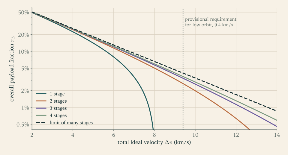
Figure 2.1 shows the whole family. Reading along the dotted line at \(9.4\ \mathrm{km/s}\) : one stage is off the bottom, two stages reach about two thirds of the many-stage limit, and three reach four fifths. For more demanding missions, further right on the chart, the curves spread apart and extra stages earn more; this is why vehicles bound for higher orbits or for escape often carry a third stage, as the Saturn V did for the Moon.
The model leaves out what each added stage costs. Every stage needs its own engines, which must start in flight, and a separation system, which must work. The Falcon 9’s manufacturer states that a two-stage architecture was chosen to minimize the number of separation events (Falcon User’s Guide; see sources). Small stages also tend to have worse structural coefficients, because some hardware does not shrink with the tanks. The launchers cited in this course use two or three stages.
Example 2.3: A real two-stage vehicle, checked against the requirement
Data. Falcon 9 stage masses from the secondary compilation used in Chapter 1 (see sources): first stage gross \(433\,100\ \mathrm{kg}\) , empty \(22\,200\ \mathrm{kg}\) ; second stage gross \(111\,500\ \mathrm{kg}\) , empty \(4000\ \mathrm{kg}\) ; second-stage specific impulse \(348\ \mathrm s\) ; maximum payload to low orbit, with no recovery of the first stage, \(22\,800\ \mathrm{kg}\) . The payload fairing is not listed and is ignored here. The compilation’s launch mass of \(549\,000\ \mathrm{kg}\) , used in Chapter 1, evidently does not include a payload this heavy; this example adds the pieces instead.
Ratios. The stacks are \(m_{0,2}=111\,500+22\,800=134\,300\ \mathrm{kg}\) and \(m_{0,1}=433\,100+134\,300=567\,400\ \mathrm{kg}\) .
| Stage 1 | Stage 2 | |
|---|---|---|
| \(\varepsilon_k\) | \(22\,200/433\,100=0.0513\) | \(4000/111\,500=0.0359\) |
| \(\lambda_k\) | \(134\,300/433\,100=0.310\) | \(22\,800/111\,500=0.204\) |
| \(\pi_k\) | \(134\,300/567\,400=0.237\) | \(22\,800/134\,300=0.170\) |
| \(m_{f,k}\) | \(567\,400-410\,900=156\,500\ \mathrm{kg}\) | \(4000+22\,800=26\,800\ \mathrm{kg}\) |
| \(\mathcal R_k\) | \(3.626\) | \(5.011\) |
The overall payload fraction is \(\pi_L=22\,800/567\,400=4.02\) percent. As a check on the identities, \((1+\lambda_1)/(\varepsilon_1+\lambda_1)=1.310/0.361=3.63\) .
Velocity. The second stage works in vacuum: \(\Delta v_2=(348)(9.80665)\ln5.011=(3412.7\ \mathrm{m/s})(1.6117)=5500\ \mathrm{m/s}\) . The first stage starts at sea level and ends in near vacuum, so its effective exhaust velocity lies between the two quoted values. Bracket it:
The vehicle’s total ideal velocity is therefore between \(9.06\) and \(9.43\ \mathrm{km/s}\) .
What this shows. A real vehicle at its maximum payload has an ideal capability right at the size of the provisional requirement used in this course, \(9.4\ \mathrm{km/s}\) , which is some reassurance about that number before Chapters 7 and 9 derive it. It also shows how the real designers divided the work: the upper stage supplies about \(5.5\ \mathrm{km/s}\) , well over half. The next section explains why that is the right direction.
2.4 The best division of velocity
A requirement \(\Delta v\) is given, along with the technology of each stage: its effective exhaust velocity \(c_k\) and its structural coefficient \(\varepsilon_k\) . The designer is free to choose how large each stage is, which amounts to choosing each mass ratio \(\mathcal R_k\) . The goal is the lightest vehicle for a given payload, that is, the smallest \(m_{0,1}/m_L=1/\pi_L\) .
The problem. Minimizing \(1/\pi_L\) is the same as minimizing its logarithm, and by Proposition 2.2
The constraint is \(\sum_kc_k\ln\mathcal R_k=\Delta v\) , and each mass ratio must lie in the interval \(1<\mathcal R_k<1/\varepsilon_k\) of Proposition 2.1.
A change of variable. Both the objective and the constraint are built from \(\ln\mathcal R_k\) , so let \(x_k=\ln\mathcal R_k\) , with \(0<x_k<\ln(1/\varepsilon_k)\) . The problem becomes
In these variables the constraint is linear. Each \(x_k\) is, up to the factor \(c_k\) , the velocity assigned to stage \(k\) .
Stationarity. Form the Lagrangian \(\mathcal L(x,\eta)=f(x)-\eta\,C(x)\) . The multiplier is written \(\eta\) in this course. Differentiating one term of \(f\) ,
so \(\partial\mathcal L/\partial x_k=0\) reads
Theorem 2.4 (optimal serial staging). Let stage \(k\) have effective exhaust velocity \(c_k>0\) and structural coefficient \(0<\varepsilon_k<1\) , and let \(\eta_{\min}=\max_k\,1/\bigl(c_k(1-\varepsilon_k)\bigr)\) . For \(\eta>\eta_{\min}\) define
If \(\Phi(\eta_{\min})<\Delta v<\sum_kc_k\ln(1/\varepsilon_k)\) , there is exactly one \(\eta>\eta_{\min}\) with \(\Phi(\eta)=\Delta v\) , and the mass ratios \(\mathcal R_k(\eta)\) are the unique minimizers of \(m_{0,1}/m_L\) subject to the velocity constraint. At the optimum
Proof. Necessity. The functions \(f\)
and \(C\)
are continuously differentiable on the open box \(0<x_k<\ln(1/\varepsilon_k)\)
, and the gradient of the constraint, \((c_1,\dots,c_N)\)
, is never zero. Under those hypotheses the Lagrange multiplier theorem of Multivariable Calculus says that at a constrained minimizer there is a number \(\eta\)
with \(\nabla f=\eta\nabla C\)
(math.multivariable-calculus.lagrange-multiplier). That is the stationarity condition derived above.
Sufficiency. The second derivative of one term of \(f\)
is \(\varepsilon e^{x}/(1-\varepsilon e^{x})^2\)
, which is positive on the box, so \(f\)
is a sum of strictly convex functions of separate variables and is strictly convex. The box is a convex set and the constraint is affine. For a convex differentiable objective with affine equality constraints, a feasible point at which the Lagrange condition holds is a global minimizer; this is the sufficiency of the Karush-Kuhn-Tucker conditions for convex problems from Continuous Optimization (math.continuous-optimization.kkt-strong-duality). Strict convexity makes the minimizer unique.
Existence of the multiplier. \(\mathcal R_k(\eta)=(1/\varepsilon_k)\bigl(1-1/(\eta c_k)\bigr)\) is less than \(1/\varepsilon_k\) for every positive \(\eta\) , exceeds \(1\) exactly when \(\eta>1/(c_k(1-\varepsilon_k))\) , and increases with \(\eta\) . So for \(\eta>\eta_{\min}\) every stage is inside its box, and \(\Phi\) is continuous and strictly increasing, rising from \(\Phi(\eta_{\min})\) toward \(\sum_kc_k\ln(1/\varepsilon_k)\) as \(\eta\to\infty\) . By the intermediate value theorem it takes each value in between exactly once.
The optimality condition deserves to be read as a designer would read it. The quantity \(1/\bigl(c_k(1-\varepsilon_k\mathcal R_k)\bigr)\) is the derivative of \(-\ln\pi_k\) with respect to \(\Delta v_k=c_kx_k\) : the fractional growth in the mass of the stack per additional metre per second asked of stage \(k\) . It is the marginal cost of velocity on that stage. The theorem says that at the optimum all stages have the same marginal cost, and that common value is \(\eta\) . If one stage were cheaper at the margin than another, shifting a little velocity onto it would lighten the vehicle. The units of \(\eta\) are \(\mathrm{s/m}\) , the reciprocal of a velocity.
The two bounds on \(\Delta v\) in the theorem have meanings too. The upper bound is the most the stages could deliver with zero payload. The lower bound matters only for small requirements: if \(\Delta v\) is below \(\Phi(\eta_{\min})\) , the best design gives some stage a mass ratio of \(1\) , which is to say it deletes that stage. Exercise 20 finds this threshold for the reference launcher.
Corollary 2.5 (identical stages share equally). If all stages have the same \(c\) and the same \(\varepsilon\) , the optimal mass ratios are all equal and each stage supplies \(\Delta v/N\) .
Proof. The formula for \(\mathcal R_k(\eta)\) depends on \(k\) only through \(c_k\) and \(\varepsilon_k\) , so equal parameters give equal mass ratios, and then \(Nc\ln\mathcal R=\Delta v\) .
This justifies the equal split used in Sections 2.2 and 2.3. The same result is obtained by direct calculation, for two stages only, in the lecture notes cited earlier (MIT 16.50 notes; see sources), which then remark that unequal stages are more complicated. With the multiplier they are not much more complicated: there is one equation in one unknown.
Common mistake. Splitting the velocity equally between stages that are not identical. Corollary 2.5 needs equal exhaust velocities and equal structural coefficients. A stage with higher \(c_k\) should take more of the velocity, and so should a stage with lower \(\varepsilon_k\) ; when the two differences pull in opposite directions, only the condition of Theorem 2.4 decides.
Solving for the multiplier. The equation \(\Phi(\eta)=\Delta v\)
has no closed-form solution in general, but \(\Phi\)
is continuous and increasing, so any bracketing method finds its root. Bisection needs only a starting interval on which \(\Phi-\Delta v\)
changes sign, and halves the interval each step; its guarantee, for a continuous function with a sign change, is in Numerical Analysis (math.numerical-analysis.root-bracketing).
Example 2.4: Dividing the velocity for the reference launcher
Inputs (illustrative design values). Two stages, both burning kerosene and liquid oxygen. Stage 1 operates from sea level to near vacuum; take a flight-average \(I_{sp,1}=300\ \mathrm s\) , so \(c_1=2942.0\ \mathrm{m/s}\) , between the \(282\) and \(311\ \mathrm s\) quoted for a real engine of this kind. Stage 2 operates in vacuum with a large nozzle; take \(I_{sp,2}=345\ \mathrm s\) , so \(c_2=3383.3\ \mathrm{m/s}\) , near the \(343\) and \(348\ \mathrm s\) of real vacuum engines (Chapter 1; see sources). Structural coefficients \(\varepsilon_1=0.06\) and \(\varepsilon_2=0.08\) , deliberately more cautious than the Falcon 9 values of Example 2.3. Requirement \(\Delta v=9400\ \mathrm{m/s}\) (provisional).
Admissible multipliers. \(1/(c_1(1-\varepsilon_1))=3.616\times10^{-4}\ \mathrm{s/m}\) and \(1/(c_2(1-\varepsilon_2))=3.213\times10^{-4}\ \mathrm{s/m}\) , so \(\eta_{\min}=3.616\times10^{-4}\ \mathrm{s/m}\) . The upper bound on velocity is \(c_1\ln(1/0.06)+c_2\ln(1/0.08)=8277+8545=16\,822\ \mathrm{m/s}\) , comfortably above the requirement.
Bisection. Try \(\eta=4.0\times10^{-4}\ \mathrm{s/m}\) : then \(\eta c_1=1.1768\) and \(\eta c_2=1.3533\) , giving \(\mathcal R_1=0.1768/(1.1768\times0.06)=2.504\) and \(\mathcal R_2=0.3533/(1.3533\times0.08)=3.263\) , so \(\Phi=2942.0\ln2.504+3383.3\ln3.263=6702\ \mathrm{m/s}\) , which is \(2698\ \mathrm{m/s}\) too little. At \(\eta=6.0\times10^{-4}\ \mathrm{s/m}\) the same computation gives \(\Phi=12\,068\ \mathrm{m/s}\) , which is \(2668\ \mathrm{m/s}\) too much. The root is bracketed.
In the table the multiplier is in units of \(10^{-4}\ \mathrm{s/m}\) and the residual \(\Phi(\eta)-\Delta v\) is in \(\mathrm{m/s}\) .
| Step | Multiplier tried | Residual | New bracket |
|---|---|---|---|
| 1 | \(5.000\) | \(+1046\) | \(4.000\) to \(5.000\) |
| 2 | \(4.500\) | \(-338\) | \(4.500\) to \(5.000\) |
| 3 | \(4.750\) | \(+430\) | \(4.500\) to \(4.750\) |
| 4 | \(4.625\) | \(+68\) | \(4.500\) to \(4.625\) |
| 5 | \(4.5625\) | \(-129\) | \(4.5625\) to \(4.625\) |
| 6 | \(4.5938\) | \(-29\) | \(4.5938\) to \(4.625\) |
| 7 | \(4.6094\) | \(+20\) | \(4.5938\) to \(4.6094\) |
| 8 | \(4.6016\) | \(-4\) | \(4.6016\) to \(4.6094\) |
Continuing to convergence, \(\eta=4.603\times10^{-4}\ \mathrm{s/m}\) .
The optimal stages. With \(\eta c_1=1.3542\) and \(\eta c_2=1.5573\) :
Checks. The velocities sum to \(4331+5069=9400\ \mathrm{m/s}\) . The marginal costs agree: \(c_1(1-\varepsilon_1\mathcal R_1)=(2942.0)(0.73846)=2172.5\ \mathrm{m/s}\) and \(c_2(1-\varepsilon_2\mathcal R_2)=(3383.3)(0.64213)=2172.5\ \mathrm{m/s}\) , both equal to \(1/\eta\) . And the answer is believable beside Example 2.3: a payload fraction of \(2.8\) percent against the real vehicle’s \(4.0\) percent, the difference being the heavier structure assumed here.
Reading the result. The upper stage takes \(54\) percent of the velocity. Its higher exhaust velocity argues for giving it more; its worse structural coefficient argues for less; the exhaust velocity wins. Compare the equal split, \(4700\ \mathrm{m/s}\) each: the payload fraction is then \(0.02787\) , lower by \(0.9\) percent of its value.
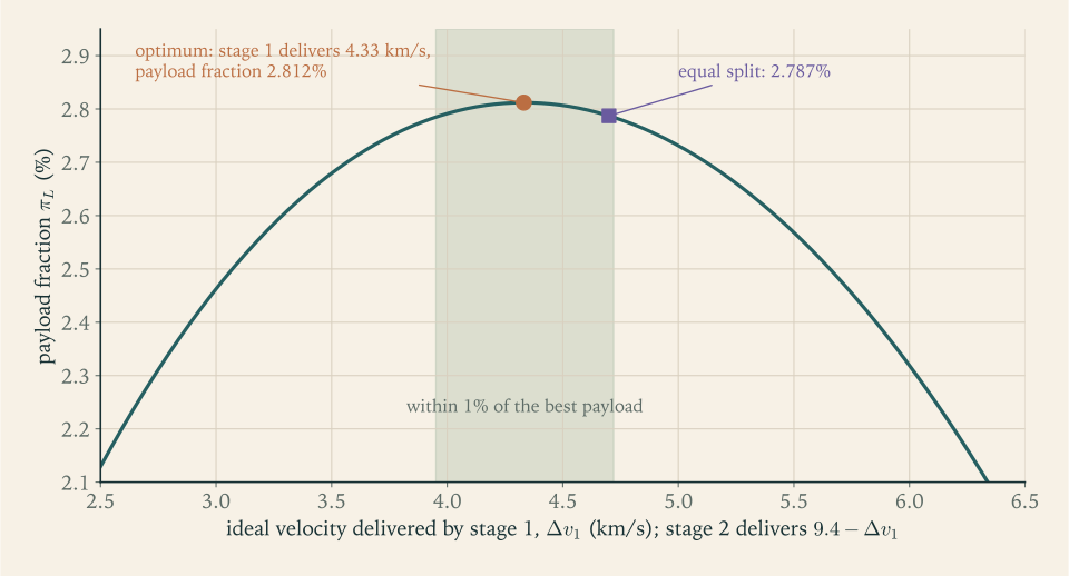
Figure 2.2 makes a point that the single number cannot. Near a smooth optimum the objective changes only to second order, so the payload is insensitive to the split over a wide band. A designer can therefore move the staging point by several hundred metres per second for other reasons, such as where the spent first stage will fall or how large an engine is available, and lose almost nothing. Outside the band the penalty grows quickly.
2.5 A first mass budget for the reference launcher
The ratios of Example 2.4 fix the shape of the vehicle. A payload mass fixes its size.
Example 2.5: Sizing the reference launcher, Revision A
Requirement. \(m_L=5000\ \mathrm{kg}\) to low orbit, with the inputs and results of Example 2.4. Thrust levels are a further design choice; take thrust-to-weight ratios at ignition of \(\psi_{0,1}=1.30\) for stage 1 and \(\psi_{0,2}=0.90\) for stage 2 (illustrative design values, discussed below).
Stack masses. Work down from the payload:
(The values printed here were computed with unrounded ratios, so recomputing from the rounded ones shown will differ in the last digits.)
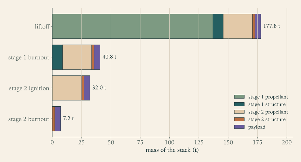
Stage masses. Stage 1 is \(m_{0,1}-m_{0,2}=145\,766\ \mathrm{kg}\) , of which \(\varepsilon_1\) is structure: \(m_{s,1}=8746\ \mathrm{kg}\) and \(m_{p,1}=137\,021\ \mathrm{kg}\) . Stage 2 is \(m_{0,2}-m_L=27\,045\ \mathrm{kg}\) : \(m_{s,2}=2164\ \mathrm{kg}\) and \(m_{p,2}=24\,881\ \mathrm{kg}\) .
| Instant | Stack mass | Composition |
|---|---|---|
| Liftoff | \(177\,812\ \mathrm{kg}\) | everything |
| Stage 1 burnout | \(40\,791\ \mathrm{kg}\) | stage 1 structure, full stage 2, payload |
| Stage 2 ignition | \(32\,045\ \mathrm{kg}\) | full stage 2, payload |
| Stage 2 burnout | \(7164\ \mathrm{kg}\) | stage 2 structure, payload |
Closure checks. \(177\,812/40\,791=4.359=\mathcal R_1\) and \(32\,045/7164=4.473=\mathcal R_2\) . The parts sum to the whole: \(137\,021+8746+24\,881+2164+5000=177\,812\ \mathrm{kg}\) .
Thrust, flow, and burn time. Treat each stage as having the single effective exhaust velocity of Example 2.4. For stage 1,
For stage 2, \(F_2=(0.90)(32\,045)(9.80665)=282.8\ \mathrm{kN}\) , \(\dot m_2=83.60\ \mathrm{kg/s}\) , and \(t_{b,2}=297.6\ \mathrm s\) .
Accelerations. By the result of Section 1.6, sensed acceleration at burnout is \(\psi_0\mathcal R\,g_0\) : \((1.30)(4.359)=5.67\,g_0\) for stage 1 and \((0.90)(4.473)=4.03\,g_0\) for stage 2.
Comparison with real vehicles. The first-stage thrust is about that of three engines of the \(845\ \mathrm{kN}\) class. The burn times are of the same order as the real timelines quoted in Chapter 1 and in the sources: \(145\) to \(155\ \mathrm s\) for first stages, and about \(360\) to \(375\ \mathrm s\) from second-stage ignition to cutoff (Falcon User’s Guide and Electron Payload User’s Guide; see sources). The liftoff mass of \(178\ \mathrm t\) for \(5\ \mathrm t\) of payload is a vehicle about a third the mass of a Falcon 9.
Two of the choices in that example need a word. A second stage with \(\psi_{0,2}\) below \(1\) could not hold itself up if it were flying vertically. It does not need to: by the time it ignites, the trajectory is nearly horizontal, the factor \(\sin\theta\) in the gravity-loss integral of Definition 1.6 is small, and what matters is finishing the burn before the vehicle falls back into the atmosphere. Low thrust means small, light engines on the stage where mass is most precious. The first stage’s \(1.30\) sits in the range computed for real vehicles in Section 1.6. Chapter 7 will test both choices by integrating the ascent.
What is provisional in this budget should be said plainly. The requirement of \(9.4\ \mathrm{km/s}\) is a placeholder. Each stage was given one exhaust velocity, although the first stage’s changes by a tenth during flight. The structural coefficients were assumed, not estimated from hardware. Nothing was set aside for a payload fairing, for propellant reserves, or for margin. Each of these is taken up in a later chapter, and each will move the numbers. What will not change is the method.
2.6 What a kilogram, a second, or a metre per second is worth
A design is only as useful as one’s knowledge of how it responds when an input changes, because every input will. There are two different questions here, and confusing them is a classic error.
The design question. Before the vehicle is built, an input changes, and the design is re-optimized. How does the liftoff mass for a given payload respond? Let \(J\) denote the optimal value of \(\ln(m_{0,1}/m_L)\) as a function of the parameters. For a constrained minimum, the derivative of the optimal value with respect to a parameter \(\xi\) equals the partial derivative of the Lagrangian with respect to \(\xi\) at the optimum. The argument is three lines. Along the family of optima, \(\mathrm dJ/\mathrm d\xi=\nabla f\cdot\mathrm dx/\mathrm d\xi+\partial f/\partial\xi\) . Differentiating the constraint gives \(\nabla C\cdot\mathrm dx/\mathrm d\xi+\partial C/\partial\xi=0\) . Since \(\nabla f=\eta\nabla C\) at the optimum, \(\mathrm dJ/\mathrm d\xi=\partial f/\partial\xi-\eta\,\partial C/\partial\xi=\partial\mathcal L/\partial\xi\) . This is the envelope property of constrained optima, treated in the Continuous Optimization course of the library.
Proposition 2.6 (design sensitivities). At the optimum of Theorem 2.4,
where \(J=\ln(m_{0,1}/m_L)\) at the optimum.
Proof. Apply \(\mathrm dJ/\mathrm d\xi=\partial\mathcal L/\partial\xi\) with \(\mathcal L=f-\eta C\) , \(C=\sum_kc_kx_k-\Delta v\) , and \(f=\sum_k[x_k+\ln(1-\varepsilon_k)-\ln(1-\varepsilon_ke^{x_k})]\) . For \(\xi=\Delta v\) only \(C\) depends on it, with \(\partial C/\partial\Delta v=-1\) . For \(\xi=c_k\) , \(\partial C/\partial c_k=x_k=\ln\mathcal R_k\) . For \(\xi=\varepsilon_k\) only \(f\) depends on it, and differentiating its \(k\) th term gives the stated expression.
So the multiplier is not just a device for finding the optimum. It is the price of velocity: the fractional increase in liftoff mass per additional metre per second of requirement. For the reference launcher \(\eta=4.603\times10^{-4}\ \mathrm{s/m}\) , so an extra \(100\ \mathrm{m/s}\) raises \(J\) by \(0.0460\) and the liftoff mass by the factor \(e^{0.0460}=1.047\) , close to 5 percent. Since \(J\) changes by \(\eta\,\delta\Delta v\) , the mass grows exponentially in the requirement with a characteristic velocity \(1/\eta=2173\ \mathrm{m/s}\) , noticeably less than either exhaust velocity. That is the staged vehicle’s version of the rocket equation’s exponential.
The other sensitivities, evaluated for the reference launcher: one more second of specific impulse changes \(c_k\) by \(g_0\) , so it changes \(J\) by \(-\eta g_0\ln\mathcal R_k\) , which is \(-0.0066\) on stage 1 and \(-0.0068\) on stage 2, about two thirds of a percent of liftoff mass per second on either stage. The structural coefficients are the most expensive inputs. The derivative \(\partial J/\partial\varepsilon_k\) is \(4.84\) for stage 1 and \(5.88\) for stage 2. Those are slopes; for a finite step, re-optimizing the design with one coefficient raised by a full \(0.01\) raises \(J\) by \(0.0474\) for stage 1 and \(0.0574\) for stage 2, which is \(4.8\) and \(5.9\) percent of liftoff mass.
The built-vehicle question. After the hardware exists, with tanks of fixed size, something changes: a component comes in overweight, or an engine underperforms. The requirement must still be met, so payload must be given up. How much? This is called an exchange ratio, and it is found by differentiating the velocity sum with the propellant loads held fixed.
Write the two-stage velocity as a function of the masses,
Adding one kilogram to the stack that stage \(k\) accelerates, with propellant fixed, changes that stage’s contribution by \(-\kappa_k\) , where
in \(\mathrm{(m/s)/kg}\) . A kilogram of payload rides on both stages and costs \(\kappa_1+\kappa_2\) . A kilogram of stage 2 structure also rides on both and costs the same, so it trades one for one with payload. A kilogram of stage 1 structure rides only on stage 1 and costs \(\kappa_1\) . Holding \(\Delta v\) fixed,
Example 2.6: Exchange ratios of the reference launcher
Coefficients. From the masses of Example 2.5,
Exchange ratios.
| Change, with tanks and requirement fixed | Payload change |
|---|---|
| \(+1\ \mathrm{kg}\) of stage 2 structure | \(-1.000\ \mathrm{kg}\) |
| \(+1\ \mathrm{kg}\) of stage 1 structure | \(-0.132\ \mathrm{kg}\) |
| \(+1\ \mathrm s\) of \(I_{sp}\) on stage 1 | \(+34.2\ \mathrm{kg}\) |
| \(+1\ \mathrm s\) of \(I_{sp}\) on stage 2 | \(+34.8\ \mathrm{kg}\) |
| \(+1\ \mathrm{m/s}\) of requirement | \(-2.37\ \mathrm{kg}\) |
Check by direct computation. Add \(100\ \mathrm{kg}\) to the stage 1 structure and solve the velocity equation numerically for the payload that restores \(9400\ \mathrm{m/s}\) : the payload falls by \(13.1\ \mathrm{kg}\) , against the linear estimate of \(13.2\ \mathrm{kg}\) . Add \(100\ \mathrm{kg}\) to stage 2 instead and the payload falls by exactly \(100\ \mathrm{kg}\) .
Reading the table. Upper-stage mass is the most expensive mass on the vehicle. First-stage mass is nearly eight times cheaper, because it is dropped at about \(4.3\ \mathrm{km/s}\) and never has to make the rest of the journey. This asymmetry explains a great deal about how launch vehicles are built: effort and cost go into lightening the upper stage, while first stages can afford robust, heavier structures and, as the Falcon 9 shows, even the hardware for recovery. One second of specific impulse is worth about \(34\ \mathrm{kg}\) of payload, some \(0.7\) percent, on either stage.
Common mistake. Quoting a design sensitivity when an exchange ratio is wanted, or the reverse, and not saying what is held fixed. For the reference launcher, “\(100\ \mathrm{m/s}\) more requirement” costs \(4.7\) percent more liftoff mass if the vehicle is redesigned around the same payload, or \(233\ \mathrm{kg}\) of payload if the vehicle is already built. Both are correct answers to different questions.
2.7 Boosters that burn alongside
Not all staging is serial. In parallel staging, boosters attached to the side of a central core ignite on the ground together with the core’s engines, burn out first, and are dropped while the core continues. The Falcon Heavy is an example: its first stage is three Falcon 9 first-stage cores side by side, 27 engines giving \(22\,819\ \mathrm{kN}\) at liftoff (Falcon User’s Guide; see sources). This section treats the idea in outline only.
The analysis proceeds by phases, each of which is an ordinary application of the rocket equation.
Phase A: boosters and core together. If the boosters have total mass flow \(\dot m_{\mathrm{boost}}\) and effective exhaust velocity \(c_{\mathrm{boost}}\) , and the core has \(\dot m_{\mathrm{core}}\) and \(c_{\mathrm{core}}\) , the vehicle’s thrust is \(\dot m_{\mathrm{boost}}c_{\mathrm{boost}}+\dot m_{\mathrm{core}}c_{\mathrm{core}}\) and its total flow is \(\dot m_{\mathrm{boost}}+\dot m_{\mathrm{core}}\) . By Definition 1.3 the effective exhaust velocity of the combination is thrust over flow,
the average of the two exhaust velocities weighted by mass flow. Phase A lasts until the boosters are empty, and its mass ratio counts the core propellant burned in that time as well.
Phase B: core alone. After the boosters’ structure is dropped, the core burns what propellant it has left.
Example 2.7: Boosters in parallel and in series
Setup (illustrative values). A core with \(100\ \mathrm t\) of propellant, \(8\ \mathrm t\) of structure, \(c_{\mathrm{core}}=3000\ \mathrm{m/s}\) , and flow \(400\ \mathrm{kg/s}\) . Two boosters, each with \(40\ \mathrm t\) of propellant, \(4\ \mathrm t\) of structure, \(c_{\mathrm{boost}}=2600\ \mathrm{m/s}\) , and flow \(400\ \mathrm{kg/s}\) . An upper stack of \(30\ \mathrm t\) rides on the core. Liftoff mass: \(108+88+30=226\ \mathrm t\) .
Parallel. The boosters empty in \(40\,000/400=100\ \mathrm s\) , during which the core burns \(40\ \mathrm t\) . In phase A,
Dropping \(8\ \mathrm t\) of booster structure leaves \(98\ \mathrm t\) ; the core’s remaining \(60\ \mathrm t\) of propellant takes it to \(38\ \mathrm t\) :
Series, for comparison. If instead the boosters burned first and the core lit only after they were dropped: \((2600)\ln(226/146)=1136.0\ \mathrm{m/s}\) , then \((3000)\ln(138/38)=3869.0\ \mathrm{m/s}\) , total \(5005.0\ \mathrm{m/s}\) .
Thrust at liftoff. In parallel the thrust is \((800)(2600)+(400)(3000)=3.28\ \mathrm{MN}\) and \(\psi_0=3.28\times10^{6}/\bigl((226\,000)(9.80665)\bigr)=1.48\) . In series the boosters alone give \(2.08\ \mathrm{MN}\) and \(\psi_0=0.94\) : the vehicle would not leave the pad.
Conclusion. On ideal velocity alone the serial arrangement is ahead by \(93.5\ \mathrm{m/s}\) , because in parallel some core propellant is spent while the boosters’ dead mass is still attached. But the serial arrangement cannot lift off, and if its boosters were enlarged until it could, they would be carrying an idle core through the densest part of the flight. Parallel burning uses every engine from the first second, which raises thrust-to-weight ratio and so cuts gravity loss (Section 1.6), and it lets all engines be started and checked on the ground. A complete comparison needs the loss terms of Chapter 7; the ideal-velocity arithmetic above is only the first entry in that ledger.
The reference launcher has no boosters, so the rest of the course uses serial staging. The phase-by-phase method is the general tool: whenever thrust, flow, or dead mass changes abruptly, start a new phase and apply the rocket equation to each.
2.8 What Revision A leaves open
The reference launcher now has numbers: \(177.8\ \mathrm t\) at liftoff, a first stage that burns \(137\ \mathrm t\) of propellant in \(178\ \mathrm s\) and supplies \(4.33\ \mathrm{km/s}\) , a second stage that burns \(24.9\ \mathrm t\) in \(298\ \mathrm s\) and supplies \(5.07\ \mathrm{km/s}\) , and \(5\ \mathrm t\) of payload. It also has a table of prices: what a second of specific impulse, a kilogram of structure on either stage, and a metre per second of requirement are each worth. Those prices say where the remaining chapters should look hardest.
Specific impulse is worth \(34\ \mathrm{kg}\) of payload per second, and so far the two values were simply assumed. Where does an exhaust velocity of three kilometres per second come from, why is it higher in vacuum than at sea level, and why does a larger nozzle raise it? Chapters 3 to 5 derive the answers from the thrust equation, the energy of the hot gas, and the flow through the nozzle. The structural coefficients, each hundredth of which is worth 5 or 6 percent of liftoff mass, are examined in Chapter 6. And the requirement itself, at \(2.4\ \mathrm{kg}\) of payload per metre per second, is the least certain input of all: Chapters 7 to 9 replace the provisional \(9.4\ \mathrm{km/s}\) by orbital speed plus computed losses.
Exercises
-
Define the structural coefficient, the payload ratio, and the payload fraction of a stage in words and in symbols. Explain why the structural coefficient is defined without the payload, and state the largest mass ratio a stage with structural coefficient \(\varepsilon\) can have and the condition under which it is attained.
-
A stage (illustrative values) has \(8\ \mathrm t\) of structure and \(92\ \mathrm t\) of propellant and carries \(20\ \mathrm t\) . Its effective exhaust velocity is \(3.2\ \mathrm{km/s}\) . (a) Compute \(\varepsilon\) , \(\lambda\) , and \(\pi\) . (b) Compute \(\mathcal R\) directly from the masses and again from \(\lambda\) and \(\varepsilon\) . (c) Compute the ideal velocity increment. (d) The carried mass is reduced to \(5\ \mathrm t\) : which of the four ratios change, and what is the new velocity increment?
Solution
The stage’s own mass is \(m_s+m_p=100\ \mathrm t\) and it carries \(m_L=20\ \mathrm t\) , so \(m_0=120\ \mathrm t\) and \(m_f=28\ \mathrm t\) .
(a) \(\varepsilon=8/100=0.08\) , \(\lambda=20/100=0.20\) , \(\pi=20/120=0.1667\) .
(b) Directly, \(\mathcal R=120/28=4.286\) . From the identity, \(\mathcal R=(1+\lambda)/(\varepsilon+\lambda)=1.20/0.28=4.286\) . The two agree, as they must; computing \(\varepsilon\) as \(8/120\) would have broken the agreement.
(c) \(\Delta v=(3.2\ \mathrm{km/s})\ln4.286=4.657\ \mathrm{km/s}\) .
(d) With \(5\ \mathrm t\) carried, \(\varepsilon\) is unchanged at \(0.08\) because the hardware is the same. The others change: \(\lambda=0.05\) , \(\pi=5/105=0.0476\) , \(\mathcal R=105/13=8.077\) , and \(\Delta v=(3.2)\ln8.077=6.685\ \mathrm{km/s}\) . The same stage gives \(2\ \mathrm{km/s}\) more when it carries a quarter of the load.
-
Some lecture notes define a stage’s structural fraction as \(\varepsilon'=m_s/m_0\) , with the stage’s initial mass including payload in the denominator (MIT 16.50 notes; see sources). (a) Show that \(\varepsilon'=\varepsilon(1-\pi)\) . (b) Show that in this convention the single-stage payload fraction is \(\pi=e^{-\Delta v/c}-\varepsilon'\) , and reconcile this with Proposition 2.1. (c) Evaluate \(\varepsilon\) and \(\varepsilon'\) for the Falcon 9 first stage using the masses of Example 2.3. (d) Explain which of the two is the better description of the hardware.
Solution
(a) Write \(\varepsilon'=m_s/m_0\) as a product: \(\dfrac{m_s}{m_s+m_p}\cdot\dfrac{m_s+m_p}{m_0}\) . The first factor is \(\varepsilon\) . The second is \((m_0-m_L)/m_0=1-\pi\) . So \(\varepsilon'=\varepsilon(1-\pi)\) .
(b) The burnout mass is \(m_f=m_s+m_L\) , so \(m_f/m_0=\varepsilon'+\pi\) . The rocket equation gives \(m_f/m_0=e^{-\Delta v/c}\) , hence \(\pi=e^{-\Delta v/c}-\varepsilon'\) . To reconcile, substitute \(\varepsilon'=\varepsilon(1-\pi)\) : \(\pi=e^{-\Delta v/c}-\varepsilon+\varepsilon\pi\) , so \(\pi(1-\varepsilon)=e^{-\Delta v/c}-\varepsilon\) , which is Proposition 2.1.
(c) \(\varepsilon=22\,200/433\,100=0.0513\) . With the \(22\,800\ \mathrm{kg}\) payload the stack is \(567\,400\ \mathrm{kg}\) , so \(\varepsilon'=22\,200/567\,400=0.0391\) ; as a check, \(\pi_1=0.2367\) and \(0.0513(1-0.2367)=0.0391\) .
(d) \(\varepsilon\) describes the hardware: it does not change when the cargo changes. \(\varepsilon'\) mixes hardware and mission, since a lighter upper stack raises it. The primed form makes the single-stage payload formula a simple difference, which is convenient on a blackboard, but a structural figure quoted for a stage should be \(\varepsilon\) .
-
For stage \(k\) of a serial vehicle, show that the structure and propellant masses are \(m_{s,k}=\varepsilon_k(1-\pi_k)\,m_{0,k}\) and \(m_{p,k}=(1-\varepsilon_k)(1-\pi_k)\,m_{0,k}\) , and use these to express the total propellant of a two-stage vehicle as a fraction of liftoff mass in terms of \(\varepsilon_1\) , \(\varepsilon_2\) , \(\pi_1\) , \(\pi_2\) .
Hint
The stage’s own mass is \(m_{0,k}-m_{0,k+1}=(1-\pi_k)m_{0,k}\) ; split it with \(\varepsilon_k\) . For the total propellant, remember that \(m_{0,2}=\pi_1m_{0,1}\) . You should reach \((1-\varepsilon_1)(1-\pi_1)+(1-\varepsilon_2)(1-\pi_2)\pi_1\) .
-
Using the Falcon 9 stage data of Example 2.3 and the vacuum exhaust velocity for the first stage, compute the vehicle’s total ideal velocity increment when the payload is \(10\,000\ \mathrm{kg}\) instead of \(22\,800\ \mathrm{kg}\) . By how much does the lighter payload raise it, and which stage gains more?
Answer
With \(10\,000\ \mathrm{kg}\) of payload, \(m_{0,2}=121\,500\ \mathrm{kg}\) and \(m_{0,1}=554\,600\ \mathrm{kg}\) ; \(\mathcal R_1=554\,600/143\,700=3.859\) and \(\mathcal R_2=121\,500/14\,000=8.679\) . Then \(\Delta v_1=4119\ \mathrm{m/s}\) , \(\Delta v_2=7374\ \mathrm{m/s}\) , total \(11\,493\ \mathrm{m/s}\) , against \(9428\ \mathrm{m/s}\) at maximum payload: a gain of \(2065\ \mathrm{m/s}\) . Stage 2 gains \(1874\ \mathrm{m/s}\) of that and stage 1 only \(191\ \mathrm{m/s}\) , because the payload is a large part of the second stage’s burnout mass and a small part of the first stage’s.
-
An analyst describes a two-stage vehicle with \(\mathcal R_1=3.6\) , \(c_1=3.0\ \mathrm{km/s}\) , \(\mathcal R_2=5.0\) , \(c_2=3.4\ \mathrm{km/s}\) and writes: “The overall mass ratio is \(\mathcal R_1\mathcal R_2=18\) and the average exhaust velocity is \(3.2\ \mathrm{km/s}\) , so \(\Delta v=3.2\ln18=9.25\ \mathrm{km/s}\) , and the vehicle’s final mass is \(1/18\) of its liftoff mass.” (a) Compute the correct \(\Delta v\) . (b) Identify the two separate errors in the analyst’s reasoning. (c) If \(\varepsilon_1=0.06\) , find the true ratio of liftoff mass to final burnout mass.
Solution
(a) Velocities add, each stage with its own exhaust velocity:
\[ \Delta v=(3.0)\ln3.6+(3.4)\ln5.0=3.843+5.472=9.315\ \mathrm{km/s}. \](b) First error: the logarithm of a product of mass ratios may be multiplied by a single exhaust velocity only when the stages share one. Here the stage with the larger logarithm also has the larger \(c\) , so a plain average undercounts; the analyst’s \(9.25\ \mathrm{km/s}\) is low by \(66\ \mathrm{m/s}\) . Second error: \(\mathcal R_1\mathcal R_2\) is not liftoff mass over final mass. \(\mathcal R_1=m_{0,1}/m_{f,1}\) and \(\mathcal R_2=m_{0,2}/m_{f,2}\) , and \(m_{0,2}\) is smaller than \(m_{f,1}\) by the dropped structure, so \(m_{0,1}/m_{f,2}=\mathcal R_1\mathcal R_2\,(m_{f,1}/m_{0,2})\) exceeds the product.
(c) With \(\varepsilon_1=0.06\) , Proposition 2.2 gives \(\pi_1=(1-0.06\times3.6)/(0.94\times3.6)=0.784/3.384=0.2317\) , so \(m_{0,2}=0.2317\,m_{0,1}\) and \(m_{f,2}=m_{0,2}/5.0=0.04634\,m_{0,1}\) . The true ratio of liftoff mass to final mass is \(1/0.04634=21.58\) , not \(18\) .
-
For two identical stages with \(a=e^{-\Delta v/(2c)}\) , show that the payload fraction exceeds that of a single stage with the same \(c\) and \(\varepsilon\) by exactly \(\varepsilon(1-a)^2/(1-\varepsilon)^2\) . Explain what the result says when \(\varepsilon=0\) and why that case is consistent with the rocket equation.
Solution
For one stage delivering the whole \(\Delta v\) , \(e^{-\Delta v/c}=a^2\) and Proposition 2.1 gives \(\pi^{(1)}=(a^2-\varepsilon)/(1-\varepsilon)\) . For two identical stages each delivering \(\Delta v/2\) , each has \(\pi_k=(a-\varepsilon)/(1-\varepsilon)\) and \(\pi^{(2)}=(a-\varepsilon)^2/(1-\varepsilon)^2\) . Put both over the denominator \((1-\varepsilon)^2\) and subtract:
\[ (a-\varepsilon)^2-(a^2-\varepsilon)(1-\varepsilon)=a^2-2a\varepsilon+\varepsilon^2-a^2+a^2\varepsilon+\varepsilon-\varepsilon^2=\varepsilon\,(1-2a+a^2)=\varepsilon\,(1-a)^2 . \]So \(\pi^{(2)}-\pi^{(1)}=\varepsilon(1-a)^2/(1-\varepsilon)^2\) , which is positive whenever \(\varepsilon\) is positive and \(\Delta v\) is not zero. Two stages always beat one.
When \(\varepsilon=0\) the difference vanishes. A stage with no structure leaves nothing behind at separation, so “two stages” is just one burn interrupted, and by the additivity of burns in Section 1.5 an interruption changes nothing. The whole benefit of staging is proportional to the dead mass available to drop. For the numbers of Example 2.2, \(a=0.2302\) and the difference is \(0.08(0.7698)^2/(0.92)^2=0.0560\) , which is \(0.0267-(-0.0293)\) .
-
Derive the many-stage limit of Proposition 2.3 in a second way. Consider a vehicle that continuously discards structure at rate \(\varepsilon/(1-\varepsilon)\) times its propellant flow, releasing it with zero relative velocity. Write the equation of motion in free space, integrate it, and show that the mass ratio needed for a given \(\Delta v\) is \(\exp\bigl(\Delta v/(c(1-\varepsilon))\bigr)\) .
Hint
Per unit time the vehicle loses propellant at \(\dot m\) and structure at \(\varepsilon\dot m/(1-\varepsilon)\) , so \(\mathrm dm/\mathrm dt=-\dot m/(1-\varepsilon)\) . Released structure has zero relative velocity and contributes no thrust, so \(m\,\mathrm dv/\mathrm dt=\dot mc\) . Eliminate \(\dot m\) to get \(m\,\mathrm dv=-c(1-\varepsilon)\,\mathrm dm\) and integrate.
-
For identical stages with \(c=3.2\ \mathrm{km/s}\) , \(\varepsilon=0.08\) , and \(\Delta v=9.4\ \mathrm{km/s}\) : (a) verify the payload fraction for three stages given in Section 2.3; (b) compute the many-stage limit; (c) find the smallest number of stages whose payload fraction is within \(15\) percent of that limit.
Answer
(a) \(e^{-9.4/9.6}=0.3756\) , \(\pi_k=(0.3756-0.08)/0.92=0.3213\) , \(\pi_L=0.3213^3=0.0332\) . (b) \(\pi_\infty=\exp(-9.4/(3.2\times0.92))=0.0411\) . (c) Three stages reach \(81\) percent of the limit and four reach \(87\) percent (\(0.0357/0.0411\) ), so four stages is the smallest number within \(15\) percent.
-
Two stages have the same effective exhaust velocity \(c\) but different structural coefficients \(\varepsilon_1\) and \(\varepsilon_2\) . (a) Use Theorem 2.4 to show that at the optimum \(\varepsilon_1\mathcal R_1=\varepsilon_2\mathcal R_2\) , and hence \(\mathcal R_1=\sqrt{e^{\Delta v/c}\,\varepsilon_2/\varepsilon_1}\) . (b) Which stage gets the larger mass ratio? (c) Evaluate the optimal mass ratios, velocity increments, and payload fraction for \(c=3.2\ \mathrm{km/s}\) , \(\varepsilon_1=0.06\) , \(\varepsilon_2=0.10\) , \(\Delta v=9.4\ \mathrm{km/s}\) , and compare the payload fraction with that of an equal split.
Solution
(a) Theorem 2.4 says \(c_k(1-\varepsilon_k\mathcal R_k)=1/\eta\) for every stage. With \(c_1=c_2=c\) this gives \(1-\varepsilon_1\mathcal R_1=1-\varepsilon_2\mathcal R_2\) , so \(\varepsilon_1\mathcal R_1=\varepsilon_2\mathcal R_2\) . The velocity constraint with equal \(c\) is \(c\ln(\mathcal R_1\mathcal R_2)=\Delta v\) , so \(\mathcal R_1\mathcal R_2=e^{\Delta v/c}\) . Substituting \(\mathcal R_2=\varepsilon_1\mathcal R_1/\varepsilon_2\) gives \(\mathcal R_1^2=e^{\Delta v/c}\varepsilon_2/\varepsilon_1\) .
(b) \(\mathcal R_1/\mathcal R_2=\varepsilon_2/\varepsilon_1\) : the stage with the smaller structural coefficient gets the larger mass ratio. A lightly built stage can be pushed harder before its structure dominates its burnout mass.
(c) \(e^{9.4/3.2}=18.87\) , so
\[ \mathcal R_1=\sqrt{18.87\times0.10/0.06}=5.608,\qquad \mathcal R_2=\sqrt{18.87\times0.06/0.10}=3.365 . \]Then \(\Delta v_1=(3.2)\ln5.608=5.517\ \mathrm{km/s}\) and \(\Delta v_2=(3.2)\ln3.365=3.883\ \mathrm{km/s}\) , which sum to \(9.400\ \mathrm{km/s}\) . The payload fractions are \(\pi_1=(1-0.3365)/(0.94\times5.608)=0.1259\) and \(\pi_2=(1-0.3365)/(0.90\times3.365)=0.2191\) , so \(\pi_L=0.02758\) . The numerators are equal, as part (a) requires.
For the equal split, both mass ratios are \(\sqrt{18.87}=4.344\) ; \(\pi_1=(1-0.2606)/(0.94\times4.344)=0.1811\) , \(\pi_2=(1-0.4344)/(0.90\times4.344)=0.1447\) , and \(\pi_L=0.02620\) . The optimal split carries \(5.3\) percent more payload.
-
Show that for a single stage \(\mathrm d(-\ln\pi_k)/\mathrm d\Delta v_k=1/\bigl(c_k(1-\varepsilon_k\mathcal R_k)\bigr)\) , and that this marginal cost increases with \(\Delta v_k\) . Use the second fact to explain, without the convexity theorem, why moving velocity from a stage with higher marginal cost to one with lower marginal cost always reduces liftoff mass.
Hint
Differentiate \(-\ln\pi_k=x_k+\ln(1-\varepsilon_k)-\ln(1-\varepsilon_ke^{x_k})\) with respect to \(x_k\) and use \(\Delta v_k=c_kx_k\) . The result increases with \(x_k\) because \(\varepsilon_ke^{x_k}\) does. For the last part, move a small \(\delta\) of velocity from stage A to stage B: the change in \(\ln(m_{0,1}/m_L)\) is \(\delta\) times (marginal cost of B minus marginal cost of A), to first order.
-
(Computation.) A three-stage vehicle (illustrative values) has \(c=(2900,\ 3300,\ 4400)\ \mathrm{m/s}\) and \(\varepsilon=(0.06,\ 0.08,\ 0.12)\) and must supply \(\Delta v=12\,000\ \mathrm{m/s}\) . Write a short program that finds the multiplier \(\eta\) by bisection or with a library root-finder, and report \(\eta\) , the three mass ratios, the three velocity increments, and the liftoff mass per kilogram of payload. Verify that \(c_k(1-\varepsilon_k\mathcal R_k)\) is the same for all three stages.
Answer
\(\eta=4.035\times10^{-4}\ \mathrm{s/m}\) . Mass ratios \(\mathcal R=(2.424,\ 3.113,\ 3.640)\) ; velocity increments \((2568,\ 3747,\ 5685)\ \mathrm{m/s}\) , summing to \(12\,000\ \mathrm{m/s}\) ; stage payload fractions \((0.3750,\ 0.2622,\ 0.1758)\) ; \(\pi_L=0.01729\) , so \(57.8\ \mathrm{kg}\) at liftoff per kilogram of payload. The common value of \(c_k(1-\varepsilon_k\mathcal R_k)\) is \(1/\eta=2478\ \mathrm{m/s}\) . The hydrogen third stage, with the highest exhaust velocity, takes nearly half the velocity despite the worst structural coefficient.
-
A designer reasons: “Corollary 2.5 says the optimum divides the velocity equally, so each stage of the reference launcher should supply \(4700\ \mathrm{m/s}\) .” (a) Say what is wrong with the reasoning. (b) Compute the payload fraction for the equal split with the inputs of Example 2.4. (c) For a \(5000\ \mathrm{kg}\) payload, how much heavier at liftoff is the equal-split vehicle than the optimal one? (d) What does the size of that penalty tell you about how carefully the split must be chosen?
Solution
(a) Corollary 2.5 applies only when the stages have the same exhaust velocity and the same structural coefficient. The reference launcher’s stages have \(c_1=2942.0\) and \(c_2=3383.3\ \mathrm{m/s}\) , and \(\varepsilon_1=0.06\) and \(\varepsilon_2=0.08\) , so the corollary does not apply and the general condition of Theorem 2.4 must be used.
(b) With \(4700\ \mathrm{m/s}\) each, \(\mathcal R_1=e^{4700/2942.0}=4.941\) and \(\mathcal R_2=e^{4700/3383.3}=4.012\) . Then
\[ \pi_1=\frac{1-(0.06)(4.941)}{(0.94)(4.941)}=0.1515,\qquad \pi_2=\frac{1-(0.08)(4.012)}{(0.92)(4.012)}=0.1840,\qquad \pi_L=0.02787 . \](c) With the unrounded fraction, liftoff mass is \(5000/0.0278722=179\,390\ \mathrm{kg}\) , against \(177\,812\ \mathrm{kg}\) for the optimum: \(1579\ \mathrm{kg}\) heavier, or \(0.9\) percent.
(d) The penalty for a \(370\ \mathrm{m/s}\) error in the split is under one percent, because the objective is flat near its minimum (Figure 2.2). The split need not be chosen to the last metre per second, and other considerations can move it within the flat region at little cost. The reasoning in the quoted argument was still wrong, and for stages that differ more, the penalty would be larger (Exercise 10 has a case costing \(5\) percent).
-
For the reference launcher, use the multiplier \(\eta=4.603\times10^{-4}\ \mathrm{s/m}\) to estimate (a) the liftoff mass, for the same payload and a re-optimized design, if the requirement rises by \(150\ \mathrm{m/s}\) ; (b) the reduction in requirement that would be worth the same as one additional second of specific impulse on stage 2. (c) The exact re-optimized liftoff mass for part (a) is \(190\,592\ \mathrm{kg}\) ; compare it with your estimate and explain the direction of the difference.
Solution
(a) By Proposition 2.6, \(\partial J/\partial\Delta v=\eta\) with \(J=\ln(m_{0,1}/m_L)\) . For a change of \(150\ \mathrm{m/s}\) , \(J\) rises by about \((4.603\times10^{-4})(150)=0.06904\) , so the liftoff mass is multiplied by \(e^{0.06904}=1.07148\) :
\[ m_{0,1}\approx(177\,812\ \mathrm{kg})(1.07148)=190\,522\ \mathrm{kg}. \](b) One second of specific impulse on stage 2 raises \(c_2\) by \(g_0\) and changes \(J\) by \(-\eta g_0\ln\mathcal R_2\) . A change \(\delta\) in the requirement changes \(J\) by \(\eta\,\delta\) . Equating, \(\delta=-g_0\ln\mathcal R_2=-(9.80665)(1.4981)=-14.7\ \mathrm{m/s}\) . A second of upper-stage specific impulse is worth a \(14.7\ \mathrm{m/s}\) reduction in the requirement.
(c) The exact value, \(190\,592\ \mathrm{kg}\) , is \(70\ \mathrm{kg}\) above the estimate. The multiplier is the slope of \(J\) at \(9400\ \mathrm{m/s}\) , and \(\eta\) itself increases with the requirement (the function \(\Phi\) of Theorem 2.4 is increasing), so \(J\) is convex in \(\Delta v\) and its tangent line lies below it. A first-order estimate from the multiplier always understates the cost of an increase.
-
For a two-stage vehicle with fixed propellant loads, derive the exchange ratio \(\partial m_L/\partial m_{s,1}=-\kappa_1/(\kappa_1+\kappa_2)\) with \(\kappa_k=c_k(1/m_{f,k}-1/m_{0,k})\) by implicit differentiation of the velocity constraint. Evaluate it for the reference launcher and find the payload lost if the first-stage structure comes in \(300\ \mathrm{kg}\) overweight.
Solution
Hold \(m_{p,1}\) , \(m_{p,2}\) , and \(m_{s,2}\) fixed and regard \(\Delta v\) as a function of \(m_L\) and \(m_{s,1}\) through \(m_{0,2}=m_{s,2}+m_{p,2}+m_L\) and \(m_{0,1}=m_{0,2}+m_{s,1}+m_{p,1}\) . For stage \(k\) , \(c_k\ln[m_{0,k}/(m_{0,k}-m_{p,k})]\) has derivative with respect to \(m_{0,k}\)
\[ c_k\left(\frac{1}{m_{0,k}}-\frac{1}{m_{0,k}-m_{p,k}}\right)=-\kappa_k . \]A change in \(m_{s,1}\) changes only \(m_{0,1}\) , so \(\partial\Delta v/\partial m_{s,1}=-\kappa_1\) . A change in \(m_L\) changes both \(m_{0,1}\) and \(m_{0,2}\) , so \(\partial\Delta v/\partial m_L=-(\kappa_1+\kappa_2)\) . Keeping \(\Delta v\) constant requires \(-\kappa_1\,\mathrm dm_{s,1}-(\kappa_1+\kappa_2)\,\mathrm dm_L=0\) , hence
\[ \frac{\partial m_L}{\partial m_{s,1}}=-\frac{\kappa_1}{\kappa_1+\kappa_2}. \]For the reference launcher, \(\kappa_1=0.05558\) and \(\kappa_2=0.36671\ \mathrm{(m/s)/kg}\) , so the ratio is \(-0.05558/0.42229=-0.1316\) . To first order an overweight of \(300\ \mathrm{kg}\) on stage 1 costs \((0.1316)(300)=39.5\ \mathrm{kg}\) of payload; solving the velocity constraint exactly for the finite change gives \(39.2\ \mathrm{kg}\) . The same overweight on stage 2 would cost \(300\ \mathrm{kg}\) .
-
A proposed upper-stage engine for the reference launcher (as built in Example 2.5, with propellant loads fixed) offers \(10\ \mathrm s\) more specific impulse but adds \(150\ \mathrm{kg}\) to the stage 2 structure. (a) Estimate the net change in payload from the exchange ratios of Example 2.6. (b) Find the added structural mass at which the new engine would exactly break even. (c) State which fixed quantities your estimate depends on.
Solution
(a) From Example 2.6, one second of specific impulse on stage 2 is worth \(+34.8\ \mathrm{kg}\) of payload and one kilogram of stage 2 structure costs one kilogram of payload. To first order the changes add:
\[ \Delta m_L\approx(10)(34.8)-150=348-150=+198\ \mathrm{kg}. \]The new engine is worth having. (Solving the velocity equation exactly with both changes gives the same \(+198\ \mathrm{kg}\) .)
(b) Break-even is where the structural penalty equals the gain: \(348\ \mathrm{kg}\) of added structure. An engine that added more than that would lose payload despite its better performance.
(c) The estimate assumes the propellant loads of both stages are fixed, the requirement stays at \(9400\ \mathrm{m/s}\) , the first stage is unchanged, and the changes are small enough for linear exchange ratios. If the vehicle could be redesigned around the new engine, the design sensitivities of Proposition 2.6 would be the right tool instead.
-
In Example 2.7 the core is throttled to half its mass flow, \(200\ \mathrm{kg/s}\) , while the boosters burn, and returns to \(400\ \mathrm{kg/s}\) afterward. Recompute \(c_{\mathrm{par}}\) , the mass at booster burnout, the velocity increments of both phases, and the liftoff thrust-to-weight ratio. Explain why the total ideal velocity rises while the liftoff thrust-to-weight ratio falls.
Answer
\(c_{\mathrm{par}}=\bigl((800)(2600)+(200)(3000)\bigr)/1000=2680\ \mathrm{m/s}\) . In \(100\ \mathrm s\) the vehicle burns \(100\ \mathrm t\) , reaching \(126\ \mathrm t\) ; \(\Delta v_A=1565.8\ \mathrm{m/s}\) . After the boosters drop, \(118\ \mathrm t\) remain with \(80\ \mathrm t\) of core propellant: \(\Delta v_B=(3000)\ln(118/38)=3399.3\ \mathrm{m/s}\) . Total \(4965.1\ \mathrm{m/s}\) , up \(53.6\ \mathrm{m/s}\) from Example 2.7. Liftoff thrust is \(2.68\ \mathrm{MN}\) and \(\psi_0=1.21\) . Throttling saves core propellant for after the dead mass is gone, which is closer to the serial arrangement; the price is lower thrust early, and therefore more gravity loss.
-
This exercise uses Chapter 1. (a) If the reference launcher’s first stage flew vertically for its whole burn with \(g=g_0\) , what would its gravity loss be, and what fraction of the stage’s ideal increment is that? (b) The second stage ignites with \(\psi_{0,2}=0.90\) . How long after ignition does its thrust-to-weight ratio reach \(1\) ? (c) Explain, using the definition of gravity loss, why a thrust-to-weight ratio below \(1\) is acceptable for the second stage but would be fatal for the first.
Solution
(a) From Example 2.5 the first stage burns for \(t_{b,1}=177.8\ \mathrm s\) . A vertical burn in uniform gravity loses \(g_0t_b\) (Definition 1.6):
\[ \Delta v_g=(9.80665\ \mathrm{m/s^2})(177.8\ \mathrm s)=1744\ \mathrm{m/s}, \]which is \(40\) percent of the stage’s ideal increment of \(4331\ \mathrm{m/s}\) . A real ascent turns away from the vertical within seconds, so this is an upper bound, but it shows that gravity loss is a first-order item in the budget.
(b) At constant thrust, \(\psi=\psi_0\,m_0/m\) , which reaches \(1\) when \(m/m_0=0.90\) , that is, when \(10\) percent of the stage 2 stack, \(3204.5\ \mathrm{kg}\) , has been burned. At \(83.60\ \mathrm{kg/s}\) that takes \(38.3\ \mathrm s\) .
(c) Gravity loss is \(\int g\sin\theta\,\mathrm dt\) . On the pad \(\theta=90^\circ\) and the vehicle has no speed: with thrust below weight it would not move at all, and all of its ideal velocity would go to gravity loss, as for the hovering lander of Exercise 1.11. The second stage ignites far above the atmosphere, already moving at several kilometres per second on a nearly horizontal path. There \(\sin\theta\) is small, so gravity removes little speed per second whatever the thrust, and the vehicle’s large horizontal speed is itself carrying it partway around the Earth. Low thrust lengthens the burn, but each second costs little.
-
The reference launcher’s customer makes two requests. (a) The payload grows to \(5500\ \mathrm{kg}\) with all ratios unchanged: find the new liftoff mass and say how each entry of the mass table in Example 2.5 changes. (b) Alternatively the liftoff mass is capped at \(177\,812\ \mathrm{kg}\) and the requirement rises to \(9500\ \mathrm{m/s}\) ; the re-optimized payload fraction is then \(0.02685\) . Find the payload, and compare the loss with the built-vehicle figure from Example 2.6.
Answer
(a) All ratios are unchanged, so every mass scales with the payload: \(m_{0,1}=(1.1)(177\,812)=195\,593\ \mathrm{kg}\) . Every entry of the mass table, and both thrusts and mass flows, scale by \(1.1\) ; ratios, velocities, burn times, and accelerations are unchanged. (b) \(m_L=(0.02685)(177\,812)=4774\ \mathrm{kg}\) , a loss of \(226\ \mathrm{kg}\) . The built vehicle of Example 2.6 loses about \(233\ \mathrm{kg}\) for the same \(100\ \mathrm{m/s}\) (the linear exchange ratio gives \(237\ \mathrm{kg}\) ): slightly more, because it cannot re-divide its propellant between the stages.
-
For the reference launcher’s stages (\(c_1=2942.0\ \mathrm{m/s}\) , \(c_2=3383.3\ \mathrm{m/s}\) , \(\varepsilon_1=0.06\) , \(\varepsilon_2=0.08\) ): (a) compute \(\eta_{\min}\) and identify which stage’s mass ratio falls to \(1\) there; (b) compute \(\Phi(\eta_{\min})\) , the smallest requirement for which the optimal design uses both stages; (c) explain in physical terms why, below that requirement, the stage identified in (a) should be left off; (d) compute the largest requirement the two stages could meet with zero payload.
Solution
(a) \(1/(c_1(1-\varepsilon_1))=1/(2942.0\times0.94)=3.616\times10^{-4}\ \mathrm{s/m}\) and \(1/(c_2(1-\varepsilon_2))=1/(3383.3\times0.92)=3.213\times10^{-4}\ \mathrm{s/m}\) . The larger is \(\eta_{\min}=3.616\times10^{-4}\ \mathrm{s/m}\) , set by stage 1, so it is the first stage whose mass ratio falls to \(1\) .
(b) At \(\eta_{\min}\) , \(\eta c_2=1.2234\) and
\[ \mathcal R_2=\frac{1.2234-1}{(1.2234)(0.08)}=2.2826,\qquad \Phi(\eta_{\min})=(3383.3\ \mathrm{m/s})\ln2.2826=2792\ \mathrm{m/s}. \](c) The marginal cost of velocity on a stage is \(1/(c_k(1-\varepsilon_k\mathcal R_k))\) , and it is lowest when the stage does almost nothing: \(1/(c_k(1-\varepsilon_k))\) . For stage 1 that floor is \(3.616\times10^{-4}\ \mathrm{s/m}\) . As long as stage 2’s marginal cost is below that floor, which is the case for requirements up to \(2792\ \mathrm{m/s}\) , every metre per second is cheaper on stage 2 and the first stage should supply none. Physically, the upper stage has the better engine, and for a small requirement its own structure is a tolerable burden; a first stage would add tanks and engines and deliver velocity at a worse price.
(d) With zero payload each stage reaches \(\mathcal R_k=1/\varepsilon_k\) : \(c_1\ln(1/0.06)+c_2\ln(1/0.08)=8277+8545=16\,822\ \mathrm{m/s}\) .