The reference launcher was sized in Chapter 2 to deliver an ideal velocity of \(9.4\ \mathrm{km/s}\) . The orbit it is going to needs a speed of about \(7.7\ \mathrm{km/s}\) . Somewhere between the pad and the orbit, \(1.7\ \mathrm{km/s}\) is expected to disappear, and so far that figure is a placeholder borrowed from other people’s vehicles. This chapter finds out where the velocity goes for this vehicle.
Three things take it. Gravity pulls back along the path for as long as the path points upward. The atmosphere resists. And thrust that is not aligned with the velocity is partly spent on turning the path instead of lengthening the velocity vector. Each of the three is an integral over the trajectory, so none can be evaluated until the trajectory is known, and the trajectory is the solution of differential equations that have no closed form once the path bends and the air thins. The plan is therefore to write the equations of motion from a free-body diagram, give them an atmosphere and a thrust model, identify the three integrals, and then integrate the whole ascent numerically, twice: once letting gravity do all the steering, and once steering the upper stage into a definite orbit.
One fact about orbits is needed before Chapter 8 derives the rest: how fast a vehicle must travel horizontally for the ground to curve away beneath it as fast as it falls. Section 7.3 obtains that speed from the equations of motion themselves.
7.1 Forces in the flight plane
The system. The vehicle is treated as a point mass \(m\) located at its centre of mass. Chapter 1 showed that the momentum balance for the closed system of vehicle plus just-expelled gas turns the engine’s effect into a force, the thrust \(F\) , acting on the vehicle; that argument was made along one line, and it holds component by component for motion in a plane, with the thrust directed along the vehicle’s axis because the exhaust leaves along that axis.
Assumptions. (i) The Earth is a sphere of radius \(R_E\) that does not rotate; its rotation is credited separately in Section 7.6. (ii) The motion stays in one plane through the Earth’s centre. (iii) The air is at rest: no wind. (iv) The vehicle is a point mass; its attitude matters only through the direction of thrust. (v) Thrust acts along the vehicle axis. (vi) Gravity is that of a point mass at the Earth’s centre, \(g=\mu_E/r^2\) with \(r=R_E+z\) .
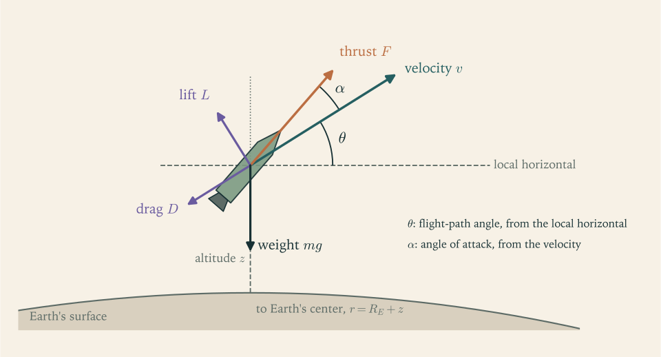
Four forces act, and Figure 7.1 shows them. Thrust \(F\) points along the vehicle axis. Drag \(D\) is the component of the aerodynamic force opposite to the velocity. Lift \(L\) is the component of the aerodynamic force perpendicular to the velocity. Weight \(mg\) points toward the Earth’s centre.
Two angles locate these forces, and both are measured in the flight plane. The flight-path angle \(\theta\) is the angle of the velocity above the local horizontal, so \(\theta=90^\circ\) is straight up and \(\theta=0\) is level flight. The angle of attack \(\alpha\) is the angle from the velocity to the vehicle axis, positive when the nose points above the velocity. With a fixed nozzle, the thrust makes the same angle \(\alpha\) with the velocity.
Common mistake. Measuring the path angle from the vertical in one equation and from the horizontal in another. Many texts, including one cited in this chapter, use the angle from the vertical, which exchanges every sine and cosine below. This course always measures \(\theta\) from the local horizontal.
The word local matters. “Horizontal” means perpendicular to the line from the Earth’s centre to the vehicle, and that line swings around as the vehicle travels downrange. Over a flight of \(1500\ \mathrm{km}\) downrange the local vertical tilts by \(1500/6378\ \mathrm{rad}\) , more than \(13^\circ\) . A frame that rotates has consequences for the equations, and the next section tracks them.
7.2 Equations of motion over a round Earth
Write the velocity as \(\mathbf v=v\,\hat{\mathbf t}\) , where \(\hat{\mathbf t}\) is the unit vector along the direction of flight, and let \(\hat{\mathbf t}_\perp\) be the unit vector perpendicular to it in the flight plane, on the side away from the Earth. Let \(\hat{\mathbf e}_r\) point from the Earth’s centre to the vehicle (local vertical) and \(\hat{\mathbf e}_x\) point horizontally downrange. Then
How fast the local frame turns. The vehicle’s horizontal velocity component is \(v\cos\theta\) , at distance \(r\) from the centre, so the line from the centre to the vehicle rotates at angular rate \(v\cos\theta/r\) . The two local unit vectors rotate with it:
The acceleration. Differentiate \(\hat{\mathbf t}\)
by the product rule for vector-valued functions of time, which holds for differentiable components as in Multivariable Calculus (math.multivariable-calculus.vector-valued-curve). The terms from \(\dot\theta\)
give \(\dot\theta\,\hat{\mathbf t}_\perp\)
. The terms from the rotating frame give \((v\cos\theta/r)(\sin\theta\,\hat{\mathbf e}_x-\cos\theta\,\hat{\mathbf e}_r)=-(v\cos\theta/r)\,\hat{\mathbf t}_\perp\)
. Hence
The quantity in parentheses is the rate at which the velocity turns as an inertial observer sees it: the rate \(\dot\theta\) at which it turns relative to the local horizontal, minus the rate at which the local horizontal itself tips forward.
The forces, resolved. Thrust is \(F(\cos\alpha\,\hat{\mathbf t}+\sin\alpha\,\hat{\mathbf t}_\perp)\) . Drag is \(-D\,\hat{\mathbf t}\) and lift is \(L\,\hat{\mathbf t}_\perp\) . Weight is \(-mg\,\hat{\mathbf e}_r\) , and inverting the relations above gives \(\hat{\mathbf e}_r=\sin\theta\,\hat{\mathbf t}+\cos\theta\,\hat{\mathbf t}_\perp\) , so weight is \(-mg\sin\theta\,\hat{\mathbf t}-mg\cos\theta\,\hat{\mathbf t}_\perp\) . Setting mass times acceleration equal to the total force and separating the two directions gives the dynamic equations. The kinematic ones are geometry: altitude grows at the vertical component of velocity, and downrange distance along the surface grows at the horizontal component scaled from radius \(r\) down to radius \(R_E\) .
Proposition 7.1 (planar ascent equations). Under assumptions (i) to (vi), with \(r=R_E+z\) and \(g=\mu_E/r^2\) ,
The state has five components, \((z,x,v,\theta,m)\) , and \(x\) feeds back into nothing: it is carried along only to report where the vehicle is.
Three checks. Dimensions: every term of the first equation is a force, and \(mv\dot\theta\) is \(\mathrm{kg\cdot(m/s)\cdot(1/s)}\) , also a force. Vertical flight: with \(\theta=90^\circ\) , \(\alpha=0\) , and \(D=L=0\) , the second equation reads \(\dot\theta=0\) and the first becomes \(m\dot v=F-mg\) , the equation of Section 1.6. Flat Earth: as \(r\to\infty\) with \(g\) held fixed the term \(v^2/r\) vanishes, and with \(\alpha=0\) and no aerodynamic force the pair reduces to \(\dot v=F/m-g\sin\theta\) and \(v\dot\theta=-g\cos\theta\) , which is the form found in introductory notes once their angle from the vertical is converted (MIT 16.07 notes; see sources).
The term that is new, compared with anything in Chapter 1, is \(mv^2\cos\theta/r\) . It did not come from a force. It came from the rotation of the local horizontal: a vehicle that moves in a straight line over a round planet sees the ground tilt away, and its path angle measured from that tilting ground increases. Section 7.3 is devoted to it.
7.3 The speed at which the ground falls away
Switch the engine off, ignore the air, and fly level: \(F=0\) , \(L=0\) , \(\theta=0\) . The second equation of Proposition 7.1 becomes
If \(v^2/r\) is less than \(g\) the path angle goes negative and the vehicle starts down. If it is greater, the vehicle starts to climb. Between the two is a speed at which the path angle stays zero: the vehicle falls, as everything in a gravitational field does, but the surface below curves away at the same rate, and its altitude does not change. With \(\theta=0\) and no drag the first equation gives \(\dot v=0\) , so the speed stays at that value too, and the motion continues indefinitely.
Definition 7.1 (circular speed). The circular speed at radius \(r\) from the Earth’s centre is the speed at which gravity supplies exactly the centripetal acceleration of a circle of that radius:
That is all of orbital mechanics this chapter needs. Whether other closed paths exist, what shape they have, and how long they take belong to Chapter 8.
The factor \(g-v^2/r\) deserves a name of its own, because it appears wherever gravity turns the path. It is the downward acceleration of the vehicle relative to the local horizon. At rest it equals \(g\) . At circular speed it is zero.
Common mistake. Reading \(g-v^2/r\) as “gravity getting weaker with altitude”. Gravity at \(400\ \mathrm{km}\) is \(89\) percent of its surface value. The subtraction is not a property of the gravitational field at all; it is the curvature of the path around the Earth, and it depends on horizontal speed, not on height.
Example 7.1: Gravity against curvature at 400 km
Question. At the altitude of the reference launcher’s target orbit, \(z=400\ \mathrm{km}\) , how large is the downward acceleration relative to the local horizon for level flight at \(2\ \mathrm{km/s}\) , at \(5\ \mathrm{km/s}\) , and at the circular speed?
Radius and gravity. \(r=6378.137+400=6778.137\ \mathrm{km}\) , using the Earth’s equatorial radius (NASA Earth Fact Sheet; see sources), and
The curvature term.
| Speed | \(v^2/r\) | \(g-v^2/r\) |
|---|---|---|
| \(2000\ \mathrm{m/s}\) | \(0.590\ \mathrm{m/s^2}\) | \(8.086\ \mathrm{m/s^2}\) |
| \(5000\ \mathrm{m/s}\) | \(3.688\ \mathrm{m/s^2}\) | \(4.988\ \mathrm{m/s^2}\) |
| \(7668.6\ \mathrm{m/s}\) | \(8.676\ \mathrm{m/s^2}\) | \(0.000\ \mathrm{m/s^2}\) |
Circular speed. \(v_{\mathrm{circ}}=\sqrt{3.986\times10^{14}/6.778137\times10^{6}}=7668.6\ \mathrm{m/s}\) , the \(7.67\ \mathrm{km/s}\) quoted since Chapter 1.
Reading the table. At \(2\ \mathrm{km/s}\) the vehicle is falling toward the horizon almost as fast as a dropped stone. At \(5\ \mathrm{km/s}\) , two thirds of orbital speed, more than half of gravity is still unbalanced, because the term goes as the square of the speed. The last kilometre per second does a disproportionate share of the work. An upper stage that is short of circular speed must hold itself up with thrust until it gets there, and that is where the remaining gravity loss of an ascent is paid.
7.4 Air: density, dynamic pressure, drag
Why density falls off exponentially. Consider a column of still air. A thin horizontal slab of thickness \(\mathrm dz\)
is held up by the difference in pressure between its lower and upper faces, which must equal its weight per unit area: \(\mathrm dp=-\rho g\,\mathrm dz\)
. If the air’s temperature is the same at all heights, its pressure is proportional to its density, \(p=\rho RT\)
, with \(R\)
the specific gas constant of air and \(T\)
the absolute temperature; this is the ideal-gas law that Chapter 4 develops. Substituting, \(\mathrm d\rho/\mathrm dz=-\rho\,g/(RT)\)
. With \(g\)
treated as constant over the few tens of kilometres that matter, the right side is a constant times \(\rho\)
, a separable first-order equation in the classification of Differential Equations (math.differential-equations.first-order-classification), and its solution is an exponential.
Definition 7.2 (exponential atmosphere). The model atmosphere of this course has density and pressure
with sea-level density \(\rho_{\mathrm{SL}}=1.217\ \mathrm{kg/m^3}\) , sea-level pressure \(p_{\mathrm{SL}}=101\,325\ \mathrm{Pa}\) , and scale height \(H=RT/g=8.5\ \mathrm{km}\) (NASA Earth Fact Sheet; see sources).
Every \(8.5\ \mathrm{km}\) of altitude divides the density by \(e\) ; every \(5.9\ \mathrm{km}\) halves it. The scale height can be checked against its formula: with \(R=286.9\ \mathrm{J/(kg\cdot K)}\) for air (NASA Glenn atmosphere model; see sources), the fact sheet’s average surface temperature of \(288\ \mathrm K\) , and \(g=9.798\ \mathrm{m/s^2}\) , \(RT/g=8.43\ \mathrm{km}\) .
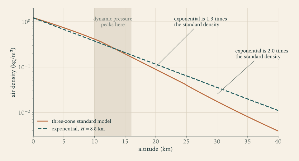
How far to trust it. The real atmosphere is not isothermal. The three-zone standard model that Section 3.4 used for pressure, in which temperature falls linearly to \(11\ \mathrm{km}\) , is constant to \(25\ \mathrm{km}\) , and rises above (NASA Glenn atmosphere model; see sources), gives the comparison below.
| Altitude | Standard-model density | Exponential density | Ratio |
|---|---|---|---|
| \(0\ \mathrm{km}\) | \(1.227\ \mathrm{kg/m^3}\) | \(1.217\ \mathrm{kg/m^3}\) | \(0.99\) |
| \(5\ \mathrm{km}\) | \(0.738\ \mathrm{kg/m^3}\) | \(0.676\ \mathrm{kg/m^3}\) | \(0.92\) |
| \(10\ \mathrm{km}\) | \(0.414\ \mathrm{kg/m^3}\) | \(0.375\ \mathrm{kg/m^3}\) | \(0.91\) |
| \(15\ \mathrm{km}\) | \(0.195\ \mathrm{kg/m^3}\) | \(0.208\ \mathrm{kg/m^3}\) | \(1.07\) |
| \(20\ \mathrm{km}\) | \(0.0890\ \mathrm{kg/m^3}\) | \(0.1157\ \mathrm{kg/m^3}\) | \(1.30\) |
| \(30\ \mathrm{km}\) | \(0.0175\ \mathrm{kg/m^3}\) | \(0.0357\ \mathrm{kg/m^3}\) | \(2.04\) |
The exponential model is within \(10\) percent up to \(15\ \mathrm{km}\) , \(30\) percent too dense at \(20\ \mathrm{km}\) , and a factor of two too dense at \(30\ \mathrm{km}\) , where the cold stratosphere has a shorter scale height than the average one. Figure 7.2 shows both models on a logarithmic scale. This error has a predictable sign: the exponential model exaggerates drag in the upper part of the atmosphere. Section 7.10 measures what that does to the answer. Above about \(80\ \mathrm{km}\) neither model is reliable, and neither needs to be, because the density is under one ten-thousandth of its sea-level value.
Dynamic pressure and drag. A body moving at speed \(v\) through air of density \(\rho\) meets, each second, a column of air of mass \(\rho v\) per unit frontal area, and must push that air aside at speeds comparable to \(v\) . The momentum it hands over per second per unit area is therefore of order \(\rho v^2\) . The conventional measure carries a factor of one half.
Definition 7.3 (dynamic pressure, drag, lift). The dynamic pressure of a flow of density \(\rho\) and speed \(v\) is \(q=\tfrac12\rho v^2\) , in pascals. The drag and lift of a body with reference area \(S\) are written
where the dimensionless drag coefficient \(C_D\) and lift coefficient \(C_L\) depend on the body’s shape, its angle of attack, and the ratio of its speed to the speed of sound.
The definition moves all the difficulty into \(C_D\) . For a launch vehicle the reference area is the body’s cross-section, and the coefficient is a few tenths: an example curve for a slender rocket rises as the vehicle passes through the speed of sound and levels off at high speed (Georgia Tech AE 4451 slides; see sources). This course uses a single constant, \(C_D=0.3\) , and a reference area \(S=7.07\ \mathrm{m^2}\) , the cross-section of a body \(3.0\ \mathrm m\) in diameter. Both are illustrative. A constant coefficient misses the rise near the speed of sound, so the model is a sizing estimate of drag and nothing more. How far it can be off is settled by data, not by the model: Example 7.6 sets its result beside published drag losses of real vehicles and finds it at the low end, by a factor of two or more against most of them.
A slender axisymmetric body flying at zero angle of attack produces no lift, by symmetry. For the rest of this chapter \(L=0\) : the vehicle flies at \(\alpha=0\) while it is in the air, and when it does take an angle of attack it is in near vacuum, where \(q\) is negligible.
Why dynamic pressure has a maximum. During ascent \(v\) increases, which raises \(q\) , and \(\rho\) decreases, which lowers it. At liftoff \(q\) is zero because \(v\) is; in space it is zero because \(\rho\) is. In between it peaks. Differentiate \(q=\tfrac12\rho_{\mathrm{SL}}e^{-z/H}v^2\) along the trajectory, using \(\dot z=v\sin\theta\) :
so the maximum occurs when \(\dot v=v^2\sin\theta/(2H)\) : the moment at which the fractional growth of \(v^2\) is exactly cancelled by the fractional thinning of the air. Engineers call this point maximum dynamic pressure, and it is the design condition for aerodynamic loads on the structure, because every aerodynamic force and bending moment scales with \(q\) .
Example 7.2: Drag on the reference launcher near maximum dynamic pressure
Flight condition. About \(70\ \mathrm s\) after liftoff the reference launcher is near \(z=12\ \mathrm{km}\) at \(v=450\ \mathrm{m/s}\) (the integration of Section 7.9 passes close to this point). Its mass is then \(177\,812-(811.1)(70)=121\,035\ \mathrm{kg}\) , using the mass flow of Section 7.5. Find the density, the dynamic pressure, and the drag, and compare the drag with the weight and with the thrust.
Density.
Dynamic pressure.
Drag. With \(C_D=0.3\) and \(S=7.07\ \mathrm{m^2}\) (illustrative),
Compared with weight and thrust. Gravity at \(12\ \mathrm{km}\) is \(9.7615\ \mathrm{m/s^2}\) , so the weight is \((121\,035)(9.7615)=1181.5\ \mathrm{kN}\) and the drag is \(5.4\) percent of it. The thrust at this altitude is \(2447\ \mathrm{kN}\) (Section 7.5), which is \(38\) times the drag.
Check. Units: \(\mathrm{(kg/m^3)(m/s)^2=kg/(m\cdot s^2)=Pa}\) , and \(\mathrm{Pa\cdot m^2=N}\) . Order of magnitude: \(30\ \mathrm{kPa}\) is about \(30\) percent of sea-level atmospheric pressure, equivalent to the weight of three tonnes on every square metre facing the flow. An independent estimate for a much smaller rocket found drag at about \(2\) percent of weight (MIT 16.07 notes; see sources); the reference launcher’s figure is higher mainly because its assumed drag coefficient and speed-density combination are larger, and both estimates say the same thing: at its worst, drag is a few percent of the forces in play.
7.5 Thrust that grows as the air thins
Chapter 1 defined thrust as \(F=\dot mv_e+(p_e-p_a)A_e\) , and Chapter 3 derived it for a control volume. The mass flow and the exit conditions are fixed by the engine, so only the term \(-p_aA_e\) changes during ascent:
Chapter 2 gave the first stage a single flight-average specific impulse of \(300\ \mathrm s\) . Chapter 3 replaced it with two values, \(I_{sp,\mathrm{SL}}=285\ \mathrm s\) at sea level and \(I_{sp,\mathrm{vac}}=315\ \mathrm s\) in vacuum (illustrative design values, bracketing the \(282\) and \(311\ \mathrm s\) quoted for a real engine in Chapter 1). Taking those as given, and keeping the liftoff thrust \(F_{\mathrm{SL}}=2267\ \mathrm{kN}\) that makes \(\psi_{0,1}=1.30\) , the first stage is described by
The burn is \(9\ \mathrm s\) shorter than Revision A’s \(177.8\ \mathrm s\) , because the same sea-level thrust at a lower sea-level specific impulse needs more flow. At \(12\ \mathrm{km}\) the ambient pressure in the model is \(24.7\ \mathrm{kPa}\) and the thrust is \(2505.5-(24.7)(2.355)=2447\ \mathrm{kN}\) : three quarters of the gain from sea level to vacuum has already been collected. The second stage works in vacuum throughout, with the constant values of Revision A: \(F_2=282.8\ \mathrm{kN}\) , \(\dot m_2=83.60\ \mathrm{kg/s}\) , \(c_2=3383.3\ \mathrm{m/s}\) .
Common mistake. Using sea-level thrust and sea-level specific impulse for the whole first-stage burn. The vehicle spends only its first minute in dense air; by the time half the propellant is gone the engine is within a few percent of its vacuum performance. The opposite error, vacuum performance from the pad, overstates the liftoff thrust-to-weight ratio by a tenth.
Since the effective exhaust velocity \(c=F/\dot m\) now varies along the path, the question of what single value to use in the rocket equation has a precise answer only after the flight is integrated. Section 7.6 defines that value and Section 7.9 computes it.
7.6 Where the ideal velocity goes
Divide the first equation of Proposition 7.1 by \(m\) , add and subtract \(F/m\) , and integrate from liftoff to engine cutoff at time \(t_{\mathrm{co}}\) .
Proposition 7.2 (the loss integrals). Along any solution of the planar ascent equations,
where
Proof. The first equation of Proposition 7.1 is \(\dot v=(F/m)\cos\alpha-D/m-g\sin\theta\) . Write \((F/m)\cos\alpha=F/m-(F/m)(1-\cos\alpha)\) and integrate each term over the burn.
The identity is exact, and it is bookkeeping, not approximation: it holds for every trajectory, optimal or foolish. The first integral is what the engines supplied. Because \(F=c\,\dot m\) and \(\dot m\,\mathrm dt=-\mathrm dm\) , it equals \(\int c\,(-\mathrm dm/m)\) , which is \(c\ln\mathcal R\) whenever \(c\) is constant, the ideal velocity increment of Chapter 1. For a stage whose \(c\) varies, define the flight-average effective exhaust velocity \(\bar c\) by \(\int(F/m)\,\mathrm dt=\bar c\,\ln\mathcal R\) ; this is exactly the single number that Chapter 2’s staging formulas need. The other three integrals are the gravity loss, the drag loss, and the steering loss.
Each has a character worth fixing in mind before any computation.
Gravity loss is paid per second, at a rate \(g\sin\theta\) . It is largest when the path is steep, and it stops when the path is level. It does not care how fast the vehicle is going, so a slow, steep start is expensive and a fast, shallow finish is nearly free. For launches to low orbit it is the largest loss by far, somewhat over a kilometre per second.
Drag loss is the time integral of \(D/m\) . Its integrand is appreciable only for the minute or so on either side of maximum dynamic pressure. Its size depends on the vehicle’s scale in a simple way. For geometrically similar vehicles, area grows as the square of length and mass as the cube, so \(S/m\) is proportional to \(m^{-1/3}\) , and on a given trajectory
A vehicle one tenth the mass loses \(10^{1/3}=2.15\) times as much velocity to drag. Small launchers suffer from the atmosphere; very large ones hardly notice it.
Steering loss is the part of the thrust acceleration that is not along the velocity. For small angles \(1-\cos\alpha\approx\alpha^2/2\) , so it is second order in the angle of attack: a few degrees cost very little, and it vanishes for a trajectory flown at \(\alpha=0\) .
Common mistake. Estimating the gravity loss of a real ascent as \(g\,t_b\) with the total burn time. For the reference launcher that would be \((9.8\ \mathrm{m/s^2})(466\ \mathrm s)=4.6\ \mathrm{km/s}\) , half the ideal velocity. The formula \(g\,t_b\) is the special case \(\theta=90^\circ\) throughout. A real path is steep for a minute or two and nearly level for the rest.
Common mistake. Adding “the energy to climb to orbital altitude” as a separate line. The climb is already inside \(\Delta v_g\) : since \(\sin\theta\,\mathrm dt=\mathrm dz/v\) , the gravity loss is \(\int g\,\mathrm dz/v\) , the velocity given up to gaining height along the actual path. A budget made of final speed plus the three losses has no place for a potential-energy term.
The rotating Earth. The equations assumed a non-rotating planet, on which the vehicle starts from rest. The real launch site moves eastward at \(\omega_ER_E\cos\phi\) , which for the reference launcher’s latitude of \(28.5^\circ\) is
(rotation rate and radius from the NASA Earth Fact Sheet; see sources). The convention of this course, and of the published budgets quoted below, is to compute the losses on a non-rotating Earth and to subtract \(\Delta v_{\mathrm{rot}}\) from the requirement as a separate line for a launch due east:
Chapter 9 tests how good that convention is and adds the terms for maneuvers in orbit.
Example 7.3: Three losses estimated by hand
Rough estimates made before a computation tell you what answer to disbelieve.
Gravity. Suppose that during the first-stage burn of \(t_{b,1}=168.9\ \mathrm s\) the sine of the path angle falls linearly from \(1\) to \(0\) , and take \(g\approx g_0\) . Then
half the \(1657\ \mathrm{m/s}\) of a vertical burn of the same length. A real path does not reach \(\theta=0\) at staging, so the true first-stage figure should lie between these two, and the upper stage will add something.
Drag. Example 7.2 found \(D/m=63.7\ \mathrm{kN}/121\,035\ \mathrm{kg}=0.526\ \mathrm{m/s^2}\) near the peak. If the drag deceleration rises to about that value and falls again over roughly \(150\ \mathrm s\) , a triangle of that base and height has area
Steering. Holding \(\alpha=5^\circ\) for \(100\ \mathrm s\) at a thrust acceleration of \(20\ \mathrm{m/s^2}\) costs
What to expect. A gravity loss of one to one and a half kilometres per second, a drag loss of tens of metres per second, and a steering loss of a few metres per second unless the angle of attack is large for a long time. If the integration returns numbers far from these, look for a bug before looking for physics.
7.7 Letting gravity do the turning
A vehicle that leaves the pad vertically and must end its burn horizontally has to rotate its velocity through \(90^\circ\) . It could do so by pointing its thrust away from its velocity, at a price in steering loss. More seriously, an angle of attack inside the atmosphere produces a sideways aerodynamic force proportional to \(q\,\alpha\) , which bends a long thin structure built to carry load along its axis. The way out is to let the weight do the turning.
Definition 7.4 (gravity turn). A gravity turn is a solution of the ascent equations with \(\alpha=0\) and \(L=0\) : thrust stays along the velocity, and the path angle obeys
The component of weight perpendicular to the velocity, less the curvature term, rotates the velocity toward the horizontal at no cost in steering loss and with no sideways load. Two features of the equation shape everything about how the maneuver is flown.
Vertical flight is an equilibrium. At \(\theta=90^\circ\)
the right side is zero. The right side is a continuously differentiable function of the state wherever \(v\)
is positive, so the initial-value problem has exactly one solution, by the existence and uniqueness theorem of Differential Equations (math.differential-equations.picard-lindelof), and since “stay vertical” is a solution it is the only one. A gravity turn started exactly vertical never turns. Gravity cannot rotate a velocity that has no horizontal component. The turn must be started by a small commanded pitch-over: at a time \(t_{\mathrm{po}}\)
shortly after liftoff the vehicle tips its velocity away from the vertical by a small angle \(\chi\)
, and only then is the angle of attack returned to zero. This chapter idealizes the pitch-over as an instantaneous rotation of the velocity by \(\chi\)
at \(t_{\mathrm{po}}=20\ \mathrm s\)
.
The equilibrium is unstable, strongly so at low speed. Let the angle from the vertical be small, write it as \(90^\circ-\theta\) , and note that \(\cos\theta\) is then that angle in radians. Near the pad \(v^2/r\) is negligible, and the gravity-turn equation says that the angle from the vertical grows at the relative rate \(g/v\) . Between two instants it is multiplied by
which for a constant net acceleration \(\dot v\) from rest, \(v=\dot v\,t\) , equals \((t_2/t_1)^{g/\dot v}\) . The reference launcher lifts off with \(\dot v=(\psi_{0,1}g_0-g)=2.95\ \mathrm{m/s^2}\) , so \(g/\dot v=3.3\) : the deviation grows roughly as the cube of the time. A pitch-over one degree too large at \(20\ \mathrm s\) is tens of degrees too large a minute later. The single number \(\chi\) therefore controls the whole shape of the trajectory, and it must be found, not guessed.
The same formula explains why the pitch-over is commanded early. At low speed the turn rate \(g\cos\theta/v\) available from gravity is large, so a small nudge suffices, and rotating a slow velocity is cheap: turning a velocity of magnitude \(v\) through an angle \(\chi\) impulsively costs \(2v\sin(\chi/2)\) , which at \(72\ \mathrm{m/s}\) and \(2^\circ\) is \(2.5\ \mathrm{m/s}\) . (The integrations below do not include this impulse. For the reference flight it is \(2.6\ \mathrm{m/s}\) ; Example 7.7 reports it where it is not small, and Chapter 9 puts it in the budget.) A vehicle that waited until it was supersonic would need a large angle of attack in dense air, the one thing the gravity turn exists to avoid.
What a gravity turn cannot do is aim. It has one free parameter. It can be adjusted to meet one condition at burnout, for example a level path, and then the burnout altitude and speed are whatever they turn out to be. Section 7.9 adds the second control needed to reach a chosen orbit.
7.8 Integrating the ascent
The method. Write the state as \(y=(z,x,v,\theta,m)\)
and the right sides of Proposition 7.1 as \(f(t,y)\)
. The classical fourth-order Runge-Kutta method of Section 1.7 advances \(y\)
by a step \(\Delta t\)
using four evaluations of \(f\)
. When \(f\)
is four times continuously differentiable along the solution, the error accumulated over a fixed interval is proportional to \((\Delta t)^4\)
; the method and its order belong to Numerical Analysis (math.numerical-analysis.ode-initial-value). The four loss integrals of Proposition 7.2 are carried as four extra components of the state whose rates are \(F/m\)
, \(g\sin\theta\)
, \(D/m\)
, and \((F/m)(1-\cos\alpha)\)
, so they are integrated by the same rule and to the same order as the trajectory.
Events. The smoothness hypothesis fails at three instants: the pitch-over, where \(\theta\) jumps by \(\chi\) ; staging, where the mass drops by \(m_{s,1}\) and the thrust and flow change; and cutoff. The remedy is to make each of these the boundary between two integrations. The flight is three smooth phases, vertical rise, first-stage turn, and second-stage burn, each divided into equal steps that end exactly on its event, and the state is edited between phases.
Common mistake. Letting a Runge-Kutta step straddle staging. The four slope evaluations then mix first-stage and second-stage right sides, the local error is no longer of fifth order, and halving the step reduces the error by about two instead of sixteen. A convergence table that shows a ratio near two is the signature of an event inside a step.
Liftoff. At \(t=0\) the speed is zero and the second equation of Proposition 7.1 would divide by it. During the vertical rise the equation is replaced by its solution, \(\theta=90^\circ\) , and only \(z\) , \(v\) , and \(m\) are advanced.
How the accuracy is judged. Integrate with a step \(\Delta t\) , then with \(\Delta t/2\) , and compare the burnout states. For a fourth-order method the difference should shrink about sixteenfold at each halving, and the last difference is an estimate of the remaining error. One step size alone proves nothing.
Finding the pitch-over angle. The burnout path angle is a function of \(\chi\)
, computed by integrating the whole flight. Requiring it to vanish is a boundary-value problem solved by shooting: guess the unknown initial datum, integrate, and correct the guess from the miss at the far end (Numerical Analysis, math.numerical-analysis.boundary-value-synthesis). With one unknown and a continuous miss function, a bracketing method such as bisection is guaranteed to converge once two guesses with misses of opposite sign are in hand (math.numerical-analysis.root-bracketing).
Example 7.4: The right-hand side at pitch-over, and one step
State. The vertical rise of the reference launcher, integrated in \(20\) steps of \(1\ \mathrm s\) , reaches \(z=673.8\ \mathrm m\) and \(v=71.90\ \mathrm{m/s}\) at \(t_{\mathrm{po}}=20\ \mathrm s\) , with mass \(m=177\,812-(811.07)(20)=161\,590\ \mathrm{kg}\) . Apply a pitch-over of \(\chi=1.9864^\circ\) (the value Example 7.5 finds), so \(\theta=88.0136^\circ\) . Evaluate the right sides of Proposition 7.1.
Forces. Ambient pressure is \((101\,325)\,e^{-673.8/8500}=93\,603\ \mathrm{Pa}\) , so
Density is \((1.217)\,e^{-0.07927}=1.1242\ \mathrm{kg/m^3}\) , dynamic pressure \(\tfrac12(1.1242)(71.90)^2=2906\ \mathrm{Pa}\) , and drag \(D=(2906)(0.3)(7.07)=6163\ \mathrm N\) . Gravity is \(g=9.7962\ \mathrm{m/s^2}\) and \(v^2/r=0.0008\ \mathrm{m/s^2}\) .
Rates.
One step. The first-stage turn lasts \(168.938-20=148.938\ \mathrm s\) ; divided into \(160\) steps, \(\Delta t=0.9309\ \mathrm s\) . One Runge-Kutta step from the state above gives
Check. The simple estimate \(\theta+\dot\theta\,\Delta t=88.0136-(0.2706)(0.9309)=87.762^\circ\) is close to the Runge-Kutta value and slightly above it, as it should be: the turn rate grows during the step because \(\cos\theta\) grows faster than \(v\) . The path is turning at more than a quarter of a degree per second from a nudge of two degrees, which is the sensitivity described in Section 7.7.
Example 7.5: The reference launcher on a gravity turn
Setup. Revision A of the reference launcher with the thrust model of Section 7.5 and the drag model of Section 7.4. Vertical rise to \(t_{\mathrm{po}}=20\ \mathrm s\) , pitch-over by \(\chi\) , gravity turn to first-stage burnout at \(168.94\ \mathrm s\) , instantaneous staging, and a second-stage gravity turn until its propellant is gone at \(466.58\ \mathrm s\) . The three phases use \(20\) , \(160\) , and \(300\) steps, each close to \(1\ \mathrm s\) . Find the \(\chi\) for which the path is level at burnout.
Shooting. Five trial angles:
| Pitch-over angle | Path angle at burnout | Altitude at burnout | Speed at burnout |
|---|---|---|---|
| \(0.5^\circ\) | \(+52.6^\circ\) | \(1048\ \mathrm{km}\) | \(5769\ \mathrm{m/s}\) |
| \(1.0^\circ\) | \(+26.8^\circ\) | \(790\ \mathrm{km}\) | \(6513\ \mathrm{m/s}\) |
| \(1.5^\circ\) | \(+10.6^\circ\) | \(499\ \mathrm{km}\) | \(7273\ \mathrm{m/s}\) |
| \(2.0^\circ\) | \(-0.25^\circ\) | \(223\ \mathrm{km}\) | \(7934\ \mathrm{m/s}\) |
| \(2.5^\circ\) | falls back into the atmosphere before burnout |
A change of two degrees at \(20\ \mathrm s\) separates a lob to a thousand kilometres from a crash. The miss changes sign between \(1.5^\circ\) and \(2.0^\circ\) . Bisection from the bracket \(1.5^\circ\) to \(2.5^\circ\) gives burnout angles \(-0.247^\circ\) at \(2.0^\circ\) , \(+4.674^\circ\) at \(1.75^\circ\) , \(+2.108^\circ\) at \(1.875^\circ\) , \(+0.906^\circ\) at \(1.9375^\circ\) , and after further halvings converges to
Convergence. Holding \(\chi\) at that value and halving the step in every phase:
| Steps in the three phases | Step size | Burnout altitude | Burnout speed |
|---|---|---|---|
| \(5,\ 40,\ 75\) | about \(4\ \mathrm s\) | \(230.787\ \mathrm{km}\) | \(7917.00\ \mathrm{m/s}\) |
| \(10,\ 80,\ 150\) | about \(2\ \mathrm s\) | \(230.619\ \mathrm{km}\) | \(7917.39\ \mathrm{m/s}\) |
| \(20,\ 160,\ 300\) | about \(1\ \mathrm s\) | \(230.606\ \mathrm{km}\) | \(7917.42\ \mathrm{m/s}\) |
| \(40,\ 320,\ 600\) | about \(0.5\ \mathrm s\) | \(230.605\ \mathrm{km}\) | \(7917.42\ \mathrm{m/s}\) |
Successive altitude differences are \(168\ \mathrm m\) , \(12.5\ \mathrm m\) , and \(0.8\ \mathrm m\) , falling by factors of about \(13\) and \(15\) , close to the sixteen expected of a fourth-order method. With \(1\ \mathrm s\) steps the burnout state is converged to about a metre in altitude and a few millimetres per second in speed, far beyond what the model’s physics deserves.
An independent formulation. A second program integrates the same forces in fixed Cartesian axes centred on the Earth, with no flight-path angle and no curvature term anywhere in it: just \(m\,\mathrm d\mathbf v/\mathrm dt\) equal to thrust along the velocity, drag against it, and gravity toward the origin. With \(1920\) steps both programs return a burnout altitude of \(230.605\ \mathrm{km}\) and a speed of \(7917.42\ \mathrm{m/s}\) . The agreement confirms the derivation of Proposition 7.1, including the term \(v^2/r\) , which the Cartesian form never mentions.
The trajectory. At first-stage burnout the vehicle is at \(z=83.3\ \mathrm{km}\) , \(127\ \mathrm{km}\) downrange, moving at \(3207\ \mathrm{m/s}\) on a path still inclined at \(21.6^\circ\) . The second stage carries it to
The losses.
| Quantity | Stage 1 | Stage 2 | Total |
|---|---|---|---|
| Ideal velocity \(\int(F/m)\,\mathrm dt\) | \(4459.0\ \mathrm{m/s}\) | \(5068.6\ \mathrm{m/s}\) | \(9527.6\ \mathrm{m/s}\) |
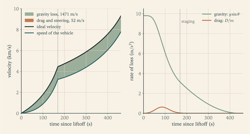
| Gravity loss | \(1206.2\ \mathrm{m/s}\) | \(358.4\ \mathrm{m/s}\) | \(1564.5\ \mathrm{m/s}\) |
| Drag loss | \(45.4\ \mathrm{m/s}\) | \(0.2\ \mathrm{m/s}\) | \(45.6\ \mathrm{m/s}\) |
| Steering loss | \(0\) | \(0\) | \(0\) |
Closure. \(9527.6-1564.5-45.6=7917.4\ \mathrm{m/s}\) , the burnout speed, as Proposition 7.2 requires.
Checks against expectation. The first-stage gravity loss of \(1206\ \mathrm{m/s}\) lies between the \(828\ \mathrm{m/s}\) and \(1657\ \mathrm{m/s}\) of Example 7.3. The drag loss of \(46\ \mathrm{m/s}\) is near the triangle estimate of \(39\ \mathrm{m/s}\) . The second stage burns for \(298\ \mathrm s\) , much longer than the first, and loses less than a third as much to gravity, because its path is shallow and its speed is high enough for \(v^2/r\) to carry much of its weight.
What the vehicle did not choose. The circular speed at \(230.6\ \mathrm{km}\) is \(\sqrt{\mu_E/r}=7766.2\ \mathrm{m/s}\) . The vehicle arrives level and \(151\ \mathrm{m/s}\) faster than that, at an altitude that was an output, not an input. Chapter 8 will show what path it then follows. A gravity turn with one parameter cannot do better; to arrive at a stated altitude with exactly circular speed takes more control.
7.9 Aiming for an orbit
Above the atmosphere the argument for \(\alpha=0\) loses its force: with negligible dynamic pressure there is no sideways load, and the only price of an angle of attack is the steering loss, which is second order. Real launch vehicles therefore fly a gravity turn, or something close to it, through the air, and steer actively in vacuum.
The simplest steering law that does the job is a constant angle of attack \(\alpha_2\) during the second-stage burn. Together with the pitch-over angle \(\chi\) and the time of engine cutoff \(t_{\mathrm{co}}\) that makes three numbers to choose, and reaching a circular orbit at a chosen altitude imposes three conditions at cutoff:
Three unknowns and three smooth conditions are a root-finding problem in three dimensions. Newton’s method, with the derivatives of the conditions with respect to the unknowns estimated by finite differences, converges quadratically from a starting point close enough to the root that the Jacobian matrix stays invertible (Numerical Analysis, math.numerical-analysis.newton-fixed-point). The gravity turn of Example 7.5 supplies such a starting point.
The target used here is a circular orbit at \(200\ \mathrm{km}\) , lower than the \(400\ \mathrm{km}\) of the requirement. The reason is in the gravity-loss integral, and Chapter 9 makes the comparison in full: climbing higher under thrust means a steeper path for longer. It is cheaper to enter a low orbit and raise it afterward.
Example 7.6: Steering the second stage into a 200 km orbit
Target. \(z=200\ \mathrm{km}\) , \(\theta=0\) , and \(v=v_{\mathrm{circ}}=\sqrt{3.986\times10^{14}/6.578137\times10^{6}}=7784.3\ \mathrm{m/s}\) .
Solution. Newton iteration on \((\chi,\alpha_2,t_{\mathrm{co}})\) , with the same step counts as before, converges to
The second stage burns for \(291.89\ \mathrm s\) of an available \(297.64\ \mathrm s\) and shuts down with \(480\ \mathrm{kg}\) of propellant unburned. Halving the step changes none of them in the first six significant figures.
The flight.
| Time | Altitude | Downrange | Speed | Path angle | Dynamic pressure | Event |
|---|---|---|---|---|---|---|
| \(20\ \mathrm s\) | \(0.67\ \mathrm{km}\) | \(0\ \mathrm{km}\) | \(72\ \mathrm{m/s}\) | \(90^\circ\) | \(2.9\ \mathrm{kPa}\) | pitch-over |
| \(40\ \mathrm s\) | \(3.07\ \mathrm{km}\) | \(0.3\ \mathrm{km}\) | \(177\ \mathrm{m/s}\) | \(78.2^\circ\) | \(13.2\ \mathrm{kPa}\) | |
| \(60\ \mathrm s\) | \(7.76\ \mathrm{km}\) | \(2.0\ \mathrm{km}\) | \(332\ \mathrm{m/s}\) | \(63.8^\circ\) | \(27.0\ \mathrm{kPa}\) | |
| \(78.5\ \mathrm s\) | \(14.4\ \mathrm{km}\) | \(6.3\ \mathrm{km}\) | \(542\ \mathrm{m/s}\) | \(50.8^\circ\) | \(32.8\ \mathrm{kPa}\) | maximum dynamic pressure |
| \(100\ \mathrm s\) | \(24.9\ \mathrm{km}\) | \(17\ \mathrm{km}\) | \(889\ \mathrm{m/s}\) | \(38.7^\circ\) | \(25.7\ \mathrm{kPa}\) | |
| \(130\ \mathrm s\) | \(44.3\ \mathrm{km}\) | \(48\ \mathrm{km}\) | \(1615\ \mathrm{m/s}\) | \(27.2^\circ\) | \(8.6\ \mathrm{kPa}\) | |
| \(168.9\ \mathrm s\) | \(78.7\ \mathrm{km}\) | \(132\ \mathrm{km}\) | \(3237\ \mathrm{m/s}\) | \(19.2^\circ\) | \(0.6\ \mathrm{kPa}\) | staging |
| \(260\ \mathrm s\) | \(155\ \mathrm{km}\) | \(440\ \mathrm{km}\) | \(3948\ \mathrm{m/s}\) | \(9.1^\circ\) | none | |
| \(400\ \mathrm s\) | \(199.5\ \mathrm{km}\) | \(1101\ \mathrm{km}\) | \(6061\ \mathrm{m/s}\) | \(0.5^\circ\) | none | |
| \(460.8\ \mathrm s\) | \(200.0\ \mathrm{km}\) | \(1504\ \mathrm{km}\) | \(7784\ \mathrm{m/s}\) | \(0.0^\circ\) | none | cutoff |
Maximum dynamic pressure. \(q_{\max}=32.8\ \mathrm{kPa}\) at \(t=78.5\ \mathrm s\) , at \(14.40\ \mathrm{km}\) and \(542\ \mathrm{m/s}\) . (The peak is flat: half a second earlier the altitude is \(0.2\ \mathrm{km}\) lower, the speed \(7\ \mathrm{m/s}\) less, and \(q\) smaller by \(5\ \mathrm{Pa}\) .) There \(\dot v=13.4\ \mathrm{m/s^2}\) and \(v^2\sin\theta/(2H)=13.4\ \mathrm{m/s^2}\) , as the condition of Section 7.4 requires. The drag is \(69.6\ \mathrm{kN}\) , which is \(6.3\) percent of the vehicle’s weight and \(2.8\) percent of its thrust at that instant.
The losses.
| Quantity | Stage 1 | Stage 2 | Total |
|---|---|---|---|
| Ideal velocity | \(4458.6\ \mathrm{m/s}\) | \(4849.0\ \mathrm{m/s}\) | \(9307.6\ \mathrm{m/s}\) |
| Gravity loss \(\Delta v_g\) | \(1173.1\ \mathrm{m/s}\) | \(297.7\ \mathrm{m/s}\) | \(1470.8\ \mathrm{m/s}\) |
| Drag loss \(\Delta v_d\) | \(48.6\ \mathrm{m/s}\) | \(0.4\ \mathrm{m/s}\) | \(49.0\ \mathrm{m/s}\) |
| Steering loss \(\Delta v_s\) | \(0\) | \(3.5\ \mathrm{m/s}\) | \(3.5\ \mathrm{m/s}\) |
Closure. \(9307.6-1470.8-49.0-3.5=7784.3\ \mathrm{m/s}\) . The steering loss agrees with the constant-angle formula: \((4849.0)(1-\cos2.178^\circ)=3.5\ \mathrm{m/s}\) .
The flight-average exhaust velocity of stage 1. The first stage’s mass ratio is \(\mathcal R_1=4.359\) , and its ideal velocity is \(4458.6\ \mathrm{m/s}\) , so
Chapter 2 assumed \(300\ \mathrm s\) , the midpoint of the sea-level and vacuum values, and Chapter 3’s rough estimate from a vertical climb was \(307\) to \(309\ \mathrm s\) . The flight average is much nearer the vacuum value of \(315\ \mathrm s\) , because the mass ratio accumulates mostly late in the burn, when the vehicle is light and already in thin air.
Accelerations. At first-stage burnout the sensed acceleration is \(F_{\mathrm{vac}}/m_{f,1}=2.5055\times10^{6}/40\,791=61.4\ \mathrm{m/s^2}\) , or \(6.26\,g_0\) , more than Revision A’s \(5.67\,g_0\) because that estimate used the sea-level thrust. At second-stage cutoff it is \(3.77\,g_0\) .
Comparison with real vehicles. Figures 7.3 and 7.4 show the flight and the accumulation of the losses. A published table of ascent budgets for six launch vehicles, computed with their real trajectories, gives the following (Georgia Tech AE 4451 slides, reproducing a table from Humble, Henry, and Larson; see sources).
| Vehicle | Gravity loss | Drag loss | Steering loss |
|---|---|---|---|
| Ariane 44L | \(1576\ \mathrm{m/s}\) | \(135\ \mathrm{m/s}\) | \(38\ \mathrm{m/s}\) |
| Atlas I | \(1395\ \mathrm{m/s}\) | \(110\ \mathrm{m/s}\) | \(167\ \mathrm{m/s}\) |
| Delta 7925 | \(1150\ \mathrm{m/s}\) | \(136\ \mathrm{m/s}\) | \(33\ \mathrm{m/s}\) |
| Space Shuttle | \(1222\ \mathrm{m/s}\) | \(107\ \mathrm{m/s}\) | \(358\ \mathrm{m/s}\) |
| Saturn V | \(1534\ \mathrm{m/s}\) | \(40\ \mathrm{m/s}\) | \(243\ \mathrm{m/s}\) |
| Titan IV with Centaur | \(1442\ \mathrm{m/s}\) | \(156\ \mathrm{m/s}\) | \(65\ \mathrm{m/s}\) |
| Reference launcher (this example) | \(1471\ \mathrm{m/s}\) | \(49\ \mathrm{m/s}\) | \(3.5\ \mathrm{m/s}\) |
The gravity loss sits in the middle of the real range. The drag loss does not: five of the six real vehicles lose between \(107\) and \(156\ \mathrm{m/s}\) to drag, with a median of \(122.5\ \mathrm{m/s}\) , and only the very large Saturn V, at \(40\ \mathrm{m/s}\) , is below the model’s \(49\ \mathrm{m/s}\) . A constant drag coefficient with no rise near the speed of sound is the likely reason, and the honest reading is that the model understates drag loss by something like a factor of two. The steering loss is far below every real value, whose median is \(116\ \mathrm{m/s}\) , and that is a statement about the model more than about the vehicle: real trajectories steer through winds, satisfy constraints on where spent stages fall, and fly vehicles whose thrust does not pass through the centre of mass. The model’s numbers are kept in what follows as the model’s numbers. A design budget must add to them, and Section 9.9 derives the addition from this table.

7.10 Trades the integration makes visible
With a program that flies the vehicle, each design choice of Chapter 2 can be tested instead of argued. In every case below the three unknowns are solved again for the same \(200\ \mathrm{km}\) orbit, and the figure of merit is the ideal velocity the engines must supply to get there.
Example 7.7: How much thrust at liftoff?
Question. Keep every mass of Revision A and change only the first stage’s thrust, so that the liftoff thrust-to-weight ratio \(\psi_{0,1}\) takes the values \(1.2\) , \(1.3\) , \(1.5\) , and \(1.7\) . The mass flow scales with the thrust and the burn time inversely. The pitch-over stays at \(20\ \mathrm s\) , and because a faster vehicle needs a larger nudge at that time, the impulse \(2v\sin(\chi/2)\) of Section 7.7 is no longer negligible and is counted here.
| \(\psi_{0,1}\) | Stage 1 burn | Pitch-over \(\chi\) | Gravity loss | Drag loss | Ideal velocity, integrated | Pitch-over impulse | Total | \(q_{\max}\) | Sensed acceleration at stage 1 burnout |
|---|---|---|---|---|---|---|---|---|---|
| \(1.2\) | \(183.0\ \mathrm s\) | \(0.47^\circ\) | \(1626\ \mathrm{m/s}\) | \(43\ \mathrm{m/s}\) | \(9459.9\ \mathrm{m/s}\) | \(0.4\ \mathrm{m/s}\) | \(9460\ \mathrm{m/s}\) | \(27.2\ \mathrm{kPa}\) | \(5.78\,g_0\) |
| \(1.3\) | \(168.9\ \mathrm s\) | \(2.10^\circ\) | \(1471\ \mathrm{m/s}\) | \(49\ \mathrm{m/s}\) | \(9307.6\ \mathrm{m/s}\) | \(2.6\ \mathrm{m/s}\) | \(9310\ \mathrm{m/s}\) | \(32.8\ \mathrm{kPa}\) | \(6.26\,g_0\) |
| \(1.5\) | \(146.4\ \mathrm s\) | \(8.90^\circ\) | \(1249\ \mathrm{m/s}\) | \(65\ \mathrm{m/s}\) | \(9099.1\ \mathrm{m/s}\) | \(17.9\ \mathrm{m/s}\) | \(9117\ \mathrm{m/s}\) | \(47.1\ \mathrm{kPa}\) | \(7.23\,g_0\) |
| \(1.7\) | \(129.2\ \mathrm s\) | \(17.57^\circ\) | \(1102\ \mathrm{m/s}\) | \(85\ \mathrm{m/s}\) | \(8971.8\ \mathrm{m/s}\) | \(48.9\ \mathrm{m/s}\) | \(9021\ \mathrm{m/s}\) | \(64.4\ \mathrm{kPa}\) | \(8.19\,g_0\) |
Reading the table. More thrust shortens the steep part of the flight and cuts the gravity loss, as Chapter 1 predicted for a vertical burn, though less sharply: from \(1.3\) to \(1.5\) the saving is \(222\ \mathrm{m/s}\) of gravity loss, against \(239\ \mathrm{m/s}\) from the vertical formula \(c\zeta/\psi_0\) with \(c=\bar c_1\) and \(\zeta=0.7706\) . Drag moves the other way, since the vehicle is faster while still low, by \(16\ \mathrm{m/s}\) , and the pitch-over impulse grows by \(15\ \mathrm{m/s}\) . The net gain in the total is \(193\ \mathrm{m/s}\) , worth about \(460\ \mathrm{kg}\) of payload at Chapter 2’s exchange ratio of \(2.37\ \mathrm{kg}\) per metre per second.
The pitch-over column is partly an artifact. The impulse is large in the last rows because the turn was started at the same time in every row, when the high-thrust vehicles are already moving at \(116\) and \(160\ \mathrm{m/s}\) . Started instead when each vehicle reaches the reference speed of \(72\ \mathrm{m/s}\) (at \(26.5\) , \(20.0\) , \(13.2\) , and \(9.7\ \mathrm s\) ), the same trajectories need pitch-over angles of \(1.35^\circ\) , \(2.10^\circ\) , \(4.31^\circ\) , and \(7.15^\circ\) and impulses of \(1.7\) , \(2.6\) , \(5.4\) , and \(9.0\ \mathrm{m/s}\) . The gain from \(1.3\) to \(1.5\) is then about \(206\ \mathrm{m/s}\) . A comparison between designs is like-for-like only when such operating choices are made the same way for each, and the table’s last column states the choice it made.
What the gain costs. Maximum dynamic pressure rises by \(43\) percent, and the structure must be built for it. The burnout acceleration passes \(7\,g_0\) . The engines are \(15\) percent larger, and engine mass is first-stage structure. Whether the trade pays depends on how heavy engines and stiffened structure are. Chapter 6 supplies the engine side: at the engine thrust-to-weight ratio of \(100\) assumed there for this stage, each kilonewton of sea-level thrust costs \(1.02\ \mathrm{kg}\) of engine, and Exercise 20 runs the trade on a figure of that size. The stiffening that a \(43\) percent higher dynamic pressure demands was not priced in Chapter 6, and it is not priced here. The two real vehicles of Section 1.6 lifted off at \(1.41\) and at between \(1.15\) and \(1.21\) .
Five further sensitivities, each obtained the same way, are worth recording.
The second stage’s thrust. With \(\psi_{0,2}\) at \(0.6\) , \(0.75\) , \(0.9\) , \(1.1\) , and \(1.3\) the ideal velocity to orbit is \(9490\) , \(9355\) , \(9308\) , \(9303\) , and \(9331\ \mathrm{m/s}\) . Below about \(0.9\) the stage cannot hold its path up without a large angle of attack, \(13^\circ\) at \(\psi_{0,2}=0.6\) , and the steering loss climbs to \(129\ \mathrm{m/s}\) . Above it nothing is gained. Chapter 2’s choice of \(0.90\) , made there by judgment, sits at the edge of a flat optimum, and the lower thrust means a lighter engine on the stage where mass is most expensive.
The drag coefficient. With \(C_D\) at \(0\) , \(0.2\) , \(0.3\) , and \(0.5\) the drag loss is \(0\) , \(33\) , \(49\) , and \(80\ \mathrm{m/s}\) and the ideal velocity to orbit is \(9237\) , \(9284\) , \(9308\) , and \(9353\ \mathrm{m/s}\) . Removing the atmosphere altogether saves \(71\ \mathrm{m/s}\) , of which \(49\) is the drag integral and the rest is gravity loss that drag caused indirectly by slowing the vehicle while its path was steep. The losses are not independent of one another. Within the model, then, an error of two thirds in the drag coefficient moves the total by half a percent. The real-vehicle data of Example 7.6 point to a larger correction than any of these coefficients gives, and Chapter 9 takes its drag allowance from the data.
The atmosphere model. Replacing the exponential atmosphere by the three-zone standard model, for both density and ambient pressure, lowers the drag loss from \(49.0\) to \(37.7\ \mathrm{m/s}\) and the ideal velocity to orbit from \(9307.6\) to \(9290.6\ \mathrm{m/s}\) , and moves maximum dynamic pressure to \(34.6\ \mathrm{kPa}\) at \(11.0\ \mathrm{km}\) . The exponential model errs by \(17\ \mathrm{m/s}\) on the cautious side.
A limit on acceleration. Chapter 3 noted that the vacuum thrust acting on the nearly empty first stage gives \(6.26\,g_0\) at burnout, more than most payloads are asked to bear. Suppose the engines are throttled from the moment \(F_{\mathrm{vac}}/m\) reaches \(5\,g_0\) , reducing the flow so that the sensed acceleration stays there. The limit is reached at \(156.2\ \mathrm s\) , when the mass is \(51\,097\ \mathrm{kg}\) ; the flow then falls in proportion to the mass, to \(80\) percent of its full value at burnout, and the stage burns out at \(170.4\ \mathrm s\) instead of \(168.9\ \mathrm s\) . The ideal velocity to orbit rises from \(9307.6\) to \(9310.7\ \mathrm{m/s}\) . A limit of \(4\,g_0\) costs \(17\ \mathrm{m/s}\) . Throttling late in a burn is cheap, because by then the path is shallow and each extra second costs little gravity loss, exactly as Exercise 1.17 anticipated. The tables of this chapter are for the unthrottled flight; a \(5\,g_0\) limit adds \(3.1\ \mathrm{m/s}\) , which Chapter 9 enters in the budget as a line of its own.
Vehicle size. A geometrically similar launcher for a \(500\ \mathrm{kg}\) payload, with every mass and thrust divided by ten and the reference area by \(10^{2/3}\) , has a drag loss of \(102.5\ \mathrm{m/s}\) , which is \(2.09\) times the reference launcher’s \(49.0\) . The scaling law of Section 7.6 predicted \(2.15\) for an unchanged trajectory; the re-solved trajectory is slightly different, which accounts for the gap.
7.11 The reference launcher after its first flight
The ascent integration revises Revision A in the following ways, all computed in this chapter for the vehicle of Chapter 2 with the thrust model of Section 7.5.
| Quantity | Value |
|---|---|
| Stage 1 mass flow, vacuum thrust, burn time | \(811.1\ \mathrm{kg/s}\) , \(2505\ \mathrm{kN}\) , \(168.9\ \mathrm s\) |
| Pitch-over at \(20\ \mathrm s\) and stage 2 angle of attack | \(2.10^\circ\) and \(2.18^\circ\) |
| Maximum dynamic pressure | \(32.8\ \mathrm{kPa}\) at \(78.5\ \mathrm s\) , altitude \(14.4\ \mathrm{km}\) , speed \(542\ \mathrm{m/s}\) |
| Staging | \(78.7\ \mathrm{km}\) altitude, \(3237\ \mathrm{m/s}\) , path angle \(19.2^\circ\) , \(132\ \mathrm{km}\) downrange |
| Insertion | circular at \(200\ \mathrm{km}\) , \(7784.3\ \mathrm{m/s}\) , \(460.8\ \mathrm s\) after liftoff |
| Gravity loss \(\Delta v_g\) | \(1470.8\ \mathrm{m/s}\) |
| Drag loss \(\Delta v_d\) | \(49.0\ \mathrm{m/s}\) |
| Steering loss \(\Delta v_s\) | \(3.5\ \mathrm{m/s}\) |
| Ideal velocity used, non-rotating Earth | \(9307.6\ \mathrm{m/s}\) |
| Flight-average exhaust velocity of stage 1 | \(3028.4\ \mathrm{m/s}\) (\(308.8\ \mathrm s\) ) |
| Sensed acceleration at stage 1 burnout | \(6.26\,g_0\) unthrottled; holding \(5\,g_0\) costs \(3.1\ \mathrm{m/s}\) |
| Pitch-over impulse, not in the integration | \(2.6\ \mathrm{m/s}\) |
On a non-rotating Earth the vehicle reaches a \(200\ \mathrm{km}\) circular orbit having spent \(9.31\ \mathrm{km/s}\) of ideal velocity, of which \(7.78\ \mathrm{km/s}\) is the speed of the orbit and \(1.52\ \mathrm{km/s}\) is loss. The provisional \(9.4\ \mathrm{km/s}\) was therefore of the right size but was not the right number, and four corrections are still to come. The Earth’s rotation will give back \(0.41\ \mathrm{km/s}\) . The orbit reached is \(200\ \mathrm{km}\) lower than the one required, and raising it costs something. The model’s drag and steering losses are smaller than real vehicles report, and the difference must be provided for. And the vehicle that flew was sized for the old number with the old exhaust velocity, so it must be resized and flown again. The first two and the last need the language of orbits: what path a vehicle follows after cutoff, what it costs to change that path, and why \(200\ \mathrm{km}\) and \(7784\ \mathrm{m/s}\) pointing level is an orbit while the same altitude at a lower speed, or the same speed tilted a few degrees, is something else. That is Chapter 8.
Where this chapter’s model stops being accurate. In order of importance for the budget: the steering model is idealized, and real steering losses are tens to hundreds of metres per second; the drag coefficient is a constant with no rise near the speed of sound, and the computed drag loss is less than half the median of the real vehicles cited; winds are ignored; the atmosphere is exponential, an error of under \(20\ \mathrm{m/s}\) ; staging is instantaneous, where real vehicles coast for several seconds; and the Earth’s rotation is handled by a credit instead of being in the equations. Chapter 10 replaces the constant angle of attack by the steering law that minimizes the ideal velocity, and Chapter 11 asks whether the vehicle can actually hold the attitudes this chapter commanded.
Exercises
-
Describe in words the free body of a launch vehicle in powered flight through the atmosphere: name the four forces, give the direction of each relative to the velocity or to the local vertical, define the flight-path angle and the angle of attack, and say which of the two dynamic equations of Proposition 7.1 each force enters and with what trigonometric factor.
Hint
Work from Figure 7.1 and the paragraph on resolving forces in Section 7.2. Thrust enters the along-path equation with \(\cos\alpha\) and the normal equation with \(\sin\alpha\) ; weight enters them with \(\sin\theta\) and \(\cos\theta\) ; drag enters only the first and lift only the second. Say from which direction each angle is measured.
-
For level flight at an altitude of \(200\ \mathrm{km}\) , compute the local gravitational acceleration, the circular speed, and the downward acceleration relative to the local horizon, \(g-v^2/r\) , at speeds of \(3\) , \(6\) , and \(7.5\ \mathrm{km/s}\) . At what speed is exactly half of gravity balanced by the curvature term?
Solution
The radius is \(r=6378.137+200=6578.137\ \mathrm{km}\) , so
\[ g=\frac{3.986\times10^{14}\ \mathrm{m^3/s^2}}{(6.578137\times10^{6}\ \mathrm m)^2}=9.212\ \mathrm{m/s^2},\qquad v_{\mathrm{circ}}=\sqrt{\frac{3.986\times10^{14}}{6.578137\times10^{6}}}=7784.3\ \mathrm{m/s}. \]The curvature term \(v^2/r\) and the net downward acceleration relative to the local horizon are:
Speed \(v^2/r\) \(g-v^2/r\) \(3\ \mathrm{km/s}\) \(1.368\ \mathrm{m/s^2}\) \(7.843\ \mathrm{m/s^2}\) \(6\ \mathrm{km/s}\) \(5.473\ \mathrm{m/s^2}\) \(3.739\ \mathrm{m/s^2}\) \(7.5\ \mathrm{km/s}\) \(8.551\ \mathrm{m/s^2}\) \(0.660\ \mathrm{m/s^2}\) Half of gravity is balanced when \(v^2/r=g/2\) , that is \(v^2=\mu_E/(2r)=v_{\mathrm{circ}}^2/2\) , so \(v=v_{\mathrm{circ}}/\sqrt2=5504\ \mathrm{m/s}\) . Because the term is quadratic in speed, a vehicle at \(71\) percent of circular speed still has half its weight unsupported, and even at \(7.5\ \mathrm{km/s}\) , \(96\) percent of circular speed, \(7\) percent remains.
-
A set of lecture notes writes the gravity turn over a flat Earth as \(\dot v=F/m-g\cos\theta_{\mathrm{vert}}\) and \(v\dot\theta_{\mathrm{vert}}=g\sin\theta_{\mathrm{vert}}\) , where \(\theta_{\mathrm{vert}}\) is the angle of the velocity from the vertical (MIT 16.07 notes; see sources). (a) Show that these follow from Proposition 7.1 with \(\alpha=0\) , \(D=L=0\) , and \(r\to\infty\) by substituting \(\theta_{\mathrm{vert}}=90^\circ-\theta\) . (b) State which term of Proposition 7.1 the flat-Earth form lacks. (c) For level flight at \(5\ \mathrm{km/s}\) at \(150\ \mathrm{km}\) altitude, compute the turning rate \(\dot\theta\) predicted by each form, in degrees per second.
Solution
(a) Put \(\alpha=0\) and \(D=L=0\) in Proposition 7.1 and let \(r\to\infty\) with \(g\) fixed, so the term \(v^2/r\) drops out: \(\dot v=F/m-g\sin\theta\) and \(v\dot\theta=-g\cos\theta\) . With \(\theta_{\mathrm{vert}}=90^\circ-\theta\) we have \(\sin\theta=\cos\theta_{\mathrm{vert}}\) , \(\cos\theta=\sin\theta_{\mathrm{vert}}\) , and \(\dot\theta_{\mathrm{vert}}=-\dot\theta\) . Substituting gives \(\dot v=F/m-g\cos\theta_{\mathrm{vert}}\) and \(v\dot\theta_{\mathrm{vert}}=g\sin\theta_{\mathrm{vert}}\) , the notes’ pair.
(b) The flat-Earth form lacks \(v^2\cos\theta/r\) , the rotation of the local horizontal. It has no circular orbit: for \(\theta=0\) it gives \(v\dot\theta=-g\) at every speed, so no horizontal speed holds altitude.
(c) At \(150\ \mathrm{km}\) , \(r=6528.137\ \mathrm{km}\) , \(g=9.353\ \mathrm{m/s^2}\) , and \(v^2/r=(5000)^2/6.528137\times10^{6}=3.830\ \mathrm{m/s^2}\) . For level flight with no thrust,
\[ \dot\theta_{\text{flat}}=-\frac{g}{v}=-\frac{9.353}{5000}\ \mathrm{rad/s}=-0.1072^\circ/\mathrm s,\qquad \dot\theta_{\text{round}}=-\frac{g-v^2/r}{v}=-\frac{5.523}{5000}\ \mathrm{rad/s}=-0.0633^\circ/\mathrm s . \]The round-Earth rate is \(59\) percent of the flat one. The flat form is adequate early in the ascent, when \(v^2/r\) is a small fraction of \(g\) , and badly wrong for an upper stage.
-
Using the exponential atmosphere and the reference launcher’s drag model (\(C_D=0.3\) , \(S=7.07\ \mathrm{m^2}\) , illustrative), compute the density, dynamic pressure, and drag (a) at \(z=8\ \mathrm{km}\) and \(v=340\ \mathrm{m/s}\) and (b) at \(z=30\ \mathrm{km}\) and \(v=1100\ \mathrm{m/s}\) . (c) The speed in (b) is more than three times that in (a); explain why the drag is nevertheless smaller.
Answer
(a) \(\rho=(1.217)e^{-8/8.5}=0.4748\ \mathrm{kg/m^3}\) , \(q=27.4\ \mathrm{kPa}\) , \(D=58.2\ \mathrm{kN}\) . (b) \(\rho=(1.217)e^{-30/8.5}=0.03569\ \mathrm{kg/m^3}\) , \(q=21.6\ \mathrm{kPa}\) , \(D=45.8\ \mathrm{kN}\) . (c) Between the two points \(v^2\) grows by a factor of \(10.5\) while the density falls by a factor of \(13.3\) ; dynamic pressure is their product, so it drops by about a fifth.
-
Derive the condition for maximum dynamic pressure, \(\dot v=v^2\sin\theta/(2H)\) , from \(q=\tfrac12\rho_{\mathrm{SL}}e^{-z/H}v^2\) . Then consider a vehicle climbing vertically with constant acceleration \(\dot v\) from rest in the exponential atmosphere: show that \(q\) peaks at altitude \(z=H\) regardless of \(\dot v\) , find the peak value in terms of \(\rho_{\mathrm{SL}}\) , \(\dot v\) , and \(H\) , and evaluate it for \(\dot v=20\ \mathrm{m/s^2}\) .
Solution
The condition. With \(\rho=\rho_{\mathrm{SL}}e^{-z/H}\) , \(\ln q=\ln(\tfrac12\rho_{\mathrm{SL}})-z/H+2\ln v\) . Differentiating along the trajectory and using \(\dot z=v\sin\theta\) ,
\[ \frac{\dot q}{q}=-\frac{v\sin\theta}{H}+\frac{2\dot v}{v}, \]which vanishes when \(\dot v=v^2\sin\theta/(2H)\) . Before that instant the second term dominates and \(q\) rises; afterward the first does.
Vertical flight at constant acceleration. Here \(\sin\theta=1\) , \(\dot v\) is constant, and from rest \(v^2=2\dot v\,z\) . The condition becomes \(\dot v=2\dot v\,z/(2H)\) , so \(z=H\) whatever the value of \(\dot v\) . Directly: \(q=\tfrac12\rho_{\mathrm{SL}}e^{-z/H}(2\dot v\,z)=\rho_{\mathrm{SL}}\,\dot v\,z\,e^{-z/H}\) , and \(ze^{-z/H}\) has its maximum \(H/e\) at \(z=H\) . Therefore
\[ q_{\max}=\frac{\rho_{\mathrm{SL}}\,\dot v\,H}{e}. \]For \(\dot v=20\ \mathrm{m/s^2}\) : \(q_{\max}=(1.217\ \mathrm{kg/m^3})(20\ \mathrm{m/s^2})(8500\ \mathrm m)/2.71828=76.1\ \mathrm{kPa}\) , reached at \(8.5\ \mathrm{km}\) and a speed of \(\sqrt{2\dot vH}=583\ \mathrm{m/s}\) .
Check. Units: \(\mathrm{(kg/m^3)(m/s^2)(m)=Pa}\) . The value is more than twice the reference launcher’s \(32.8\ \mathrm{kPa}\) , as expected: the reference launcher accelerates at well under \(20\ \mathrm{m/s^2}\) in the lower atmosphere, and the peak value is proportional to the acceleration.
-
Starting from the balance \(\mathrm dp=-\rho g\,\mathrm dz\) and \(p=\rho RT\) with constant \(T\) and \(g\) : (a) derive \(\rho(z)=\rho_{\mathrm{SL}}e^{-z/H}\) and identify \(H\) ; (b) show that the mass of air above altitude \(z\) per unit area of ground is \(\rho_{\mathrm{SL}}He^{-z/H}\) and evaluate it at sea level; (c) compare the weight of that column per unit area with the sea-level pressure of the model and explain any difference; (d) find the fraction of the atmosphere’s mass that lies below \(14.4\ \mathrm{km}\) , where the reference launcher meets maximum dynamic pressure.
Solution
(a) Substituting \(p=\rho RT\) into \(\mathrm dp=-\rho g\,\mathrm dz\) with \(T\) constant gives \(RT\,\mathrm d\rho=-\rho g\,\mathrm dz\) , a separable equation: \(\mathrm d\rho/\rho=-\mathrm dz/H\) with \(H=RT/g\) . Integrating from sea level, \(\ln(\rho/\rho_{\mathrm{SL}})=-z/H\) , so \(\rho=\rho_{\mathrm{SL}}e^{-z/H}\) .
(b) The mass above altitude \(z\) per unit ground area is
\[ \int_z^\infty\rho_{\mathrm{SL}}e^{-z'/H}\,\mathrm dz'=\rho_{\mathrm{SL}}He^{-z/H}, \]and at sea level this is \((1.217\ \mathrm{kg/m^3})(8500\ \mathrm m)=10\,344.5\ \mathrm{kg/m^2}\) : ten tonnes of air stand over every square metre.
(c) Its weight per unit area, with \(g=9.798\ \mathrm{m/s^2}\) , is \(101\,358\ \mathrm{Pa}\) , which exceeds the model’s sea-level pressure of \(101\,325\ \mathrm{Pa}\) by \(0.03\) percent. They should agree, because hydrostatic balance says the pressure at the bottom of a column equals the weight of the column per unit area. The tiny difference reflects the rounding of the tabulated density and scale height and the neglect of the weakening of gravity with height.
(d) The fraction of the mass below \(z\) is \(1-e^{-z/H}=1-e^{-14.4/8.5}=0.816\) . At maximum dynamic pressure the vehicle is already above four fifths of the atmosphere.
-
This exercise uses Chapters 1 and 3. For the reference launcher’s first stage (\(\dot m_1=811.1\ \mathrm{kg/s}\) , \(F_{\mathrm{vac}}=2505.5\ \mathrm{kN}\) , \(A_e=2.355\ \mathrm{m^2}\) ) compute the thrust and the specific impulse at sea level, at \(10\ \mathrm{km}\) , and at \(30\ \mathrm{km}\) in the exponential atmosphere, and the fraction of the sea-level-to-vacuum thrust gain that has been collected at each altitude.
Answer
Since \(F=F_{\mathrm{vac}}-p_aA_e\) and \(p_a=p_{\mathrm{SL}}e^{-z/H}\) , the fraction of the gain collected at altitude \(z\) is \(1-e^{-z/H}\) . Sea level: \(p_a=101.3\ \mathrm{kPa}\) , \(F=2266.9\ \mathrm{kN}\) , \(I_{sp}=285.0\ \mathrm s\) , fraction \(0\) . At \(10\ \mathrm{km}\) : \(p_a=31.2\ \mathrm{kPa}\) , \(F=2431.9\ \mathrm{kN}\) , \(I_{sp}=305.7\ \mathrm s\) , fraction \(0.69\) . At \(30\ \mathrm{km}\) : \(p_a=2.97\ \mathrm{kPa}\) , \(F=2498.5\ \mathrm{kN}\) , \(I_{sp}=314.1\ \mathrm s\) , fraction \(0.97\) .
-
A student estimates the gravity loss of the reference ascent as follows: “The engines burn for \(461\ \mathrm s\) and \(g\) is about \(9.5\ \mathrm{m/s^2}\) on average, so the loss is \(4.4\ \mathrm{km/s}\) .” (a) State the error. (b) Using the flight table of Example 7.6, estimate \(\int g\sin\theta\,\mathrm dt\) over the first stage by the trapezoidal rule on the tabulated path angles with \(g=9.7\ \mathrm{m/s^2}\) , and compare with the computed \(1173\ \mathrm{m/s}\) . (c) Explain why the second stage, which burns longer, loses much less.
Solution
(a) The product \(g\,t_b\) is the gravity loss only if \(\sin\theta=1\) for the whole burn, that is, for a vertical flight. The definition is \(\Delta v_g=\int g\sin\theta\,\mathrm dt\) , and for most of this ascent \(\sin\theta\) is far below one.
(b) From the flight table, with \(\theta=90^\circ\) from liftoff to \(20\ \mathrm s\) , the sines of the tabulated path angles at \(0\) , \(20\) , \(40\) , \(60\) , \(78\) , \(100\) , \(130\) , and \(168.9\ \mathrm s\) are \(1\) , \(1\) , \(0.9789\) , \(0.8973\) , \(0.7760\) , \(0.6252\) , \(0.4571\) , and \(0.3289\) . The trapezoidal rule gives
\[ \int_0^{168.9}\sin\theta\,\mathrm dt\approx20.00+19.79+18.76+15.06+15.41+16.24+15.29=120.5\ \mathrm s, \]so \(\Delta v_g\approx(9.7\ \mathrm{m/s^2})(120.5\ \mathrm s)=1169\ \mathrm{m/s}\) , within half a percent of the computed \(1173\ \mathrm{m/s}\) . The burn lasts \(169\ \mathrm s\) but counts as only \(120\) “vertical seconds”.
(c) During the second stage’s \(292\ \mathrm s\) the path angle falls from \(19^\circ\) to zero, so \(\sin\theta\) averages about a tenth: \(297.7/(9.3\times292)=0.11\) . The loss rate depends on the steepness of the path, not on how hard gravity pulls; \(g\) itself has dropped only \(6\) percent at \(200\ \mathrm{km}\) .
-
Suppose the path angle of a first stage decreases linearly in time from \(90^\circ\) to \(0\) over a burn of duration \(t_b\) , with constant \(g\) . (a) Show that \(\Delta v_g=(2/\pi)\,g\,t_b\) . (b) Compare with the result when \(\sin\theta\) , instead of \(\theta\) , decreases linearly. (c) Which of the two profiles spends more time near the vertical, and how does the comparison of the two losses reflect that?
Solution
(a) Let \(\theta(t)=\tfrac\pi2(1-t/t_b)\) . With the substitution \(s=t/t_b\) ,
\[ \Delta v_g=g\int_0^{t_b}\sin\Bigl[\tfrac\pi2\Bigl(1-\frac t{t_b}\Bigr)\Bigr]\mathrm dt=g\,t_b\int_0^1\cos\Bigl(\frac{\pi s}{2}\Bigr)\mathrm ds=g\,t_b\,\frac2\pi=0.6366\,g\,t_b . \](b) When \(\sin\theta\) falls linearly the integral is \(\tfrac12g\,t_b\) (Example 7.3). The linear-angle profile loses \((2/\pi)/(1/2)=1.27\) times as much. For the reference launcher’s first-stage burn of \(168.9\ \mathrm s\) with \(g=g_0\) the two estimates are \(1054\ \mathrm{m/s}\) and \(828\ \mathrm{m/s}\) .
(c) The sine of an angle near \(90^\circ\) changes slowly with the angle, so a path whose angle decreases at a steady rate keeps \(\sin\theta\) close to one for a long time: at the halfway point \(\theta=45^\circ\) and \(\sin\theta=0.71\) , against \(0.5\) for the other profile. More time near the vertical means more loss. The computed first-stage loss of the gravity turn, about \(1200\ \mathrm{m/s}\) , is above both estimates because the real path does not reach the horizontal by staging.
-
A stage flies its whole burn at a constant angle of attack \(\alpha\) . (a) Show from Proposition 7.2 that its steering loss is \((1-\cos\alpha)\) times its ideal velocity increment. (b) Evaluate the loss for the second stage of Example 7.6, whose ideal increment is \(4849.0\ \mathrm{m/s}\) at \(\alpha_2=2.178^\circ\) . (c) Evaluate it for \(\alpha=13^\circ\) and an ideal increment of \(5000\ \mathrm{m/s}\) . (d) By what factor does the loss grow when the angle is doubled, for small angles?
Solution
(a) With \(\alpha\) constant, \(1-\cos\alpha\) comes outside the integral of Proposition 7.2:
\[ \Delta v_s=(1-\cos\alpha)\int_0^{t_b}\frac Fm\,\mathrm dt=(1-\cos\alpha)\,\Delta v_{\mathrm{ideal}} . \](b) \((4849.0\ \mathrm{m/s})(1-\cos2.178^\circ)=(4849.0)(7.224\times10^{-4})=3.50\ \mathrm{m/s}\) , the steering loss of Example 7.6.
(c) \(1-\cos13^\circ=0.02563\) , so the loss is \((5000\ \mathrm{m/s})(0.02563)=128\ \mathrm{m/s}\) .
(d) For small angles \(1-\cos\alpha\approx\alpha^2/2\) , so doubling the angle multiplies the loss by four. Between (b) and (c) the angle grew sixfold and the loss per unit of ideal velocity by a factor of \(35\) , close to \(6^2\) . Steering loss is negligible for a couple of degrees and expensive beyond ten.
-
Two launch vehicles are geometrically similar and fly the same trajectory with the same drag coefficient; the second has one tenth the mass of the first. (a) Show that the ratio of their drag accelerations \(D/m\) at every instant is \(10^{1/3}\) . (b) Section 7.10 reports \(102.5\ \mathrm{m/s}\) and \(49.0\ \mathrm{m/s}\) for such a pair; compute the ratio and explain why it is not exactly \(10^{1/3}\) . (c) Estimate the drag loss of a similar vehicle with ten times the reference launcher’s mass.
Answer
(a) \(D/m=qC_DS/m\) ; on the same trajectory \(q\) and \(C_D\) are the same, and for similar shapes \(S\propto m^{2/3}\) , so \(D/m\propto m^{-1/3}\) and the ratio is \(10^{1/3}=2.15\) . (b) \(102.5/49.0=2.09\) . The smaller vehicle, slowed more by drag, is re-aimed onto a slightly different path, which is a little slower through the dense air, so its drag integral grows by less than the scaling law predicts. (c) About \(49.0\times10^{-1/3}=23\ \mathrm{m/s}\) .
-
This exercise uses Chapter 1. A vehicle burns vertically from rest in uniform gravity \(g\) with constant thrust and exhaust velocity, reaching speed \(v_b=c\ln\mathcal R-g\,t_b\) at altitude \(z_b\) . A colleague proposes to “correct” the burnout speed for the climb by subtracting \(\sqrt{2gz_b}\) as well. (a) Using the equation of motion, show that \(\tfrac12v_b^2+gz_b=\int_0^{t_b}(F/m)\,v\,\mathrm dt\) , so that the engine’s work accounts for both the kinetic and the potential energy with nothing left over. (b) Explain in one or two sentences why the gravity loss \(g\,t_b\) already contains the cost of the climb. (c) For Example 1.4 (\(v_b=2351\ \mathrm{m/s}\) , \(z_b=112.1\ \mathrm{km}\) , \(g=g_0\) ) compute what the colleague’s doubly corrected speed would be and say what is wrong with it.
Solution
(a) The vertical equation of motion is \(\dot v=F/m-g\) . Multiply by \(v=\dot z\) :
\[ v\,\dot v+g\,\dot z=\frac Fm\,v\qquad\Longrightarrow\qquad\frac{\mathrm d}{\mathrm dt}\Bigl(\tfrac12v^2+gz\Bigr)=\frac Fm\,v . \]Integrating from rest at the ground gives \(\tfrac12v_b^2+gz_b=\int_0^{t_b}(F/m)\,v\,\mathrm dt\) . The right side is the work done by the thrust per unit of vehicle mass along the path. It accounts for the kinetic energy and the potential energy together; no third term appears.
(b) The speed \(v_b=c\ln\mathcal R-g\,t_b\) is the solution of the same equation of motion, so it is the actual burnout speed at the actual burnout altitude. The term \(g\,t_b\) is the velocity that gravity removed while the vehicle was climbing; since \(g\,\mathrm dt=g\,\mathrm dz/v\) , it is the cost of the climb expressed in velocity units.
(c) For Example 1.4, \(\tfrac12v_b^2=2.76\ \mathrm{MJ/kg}\) and \(g_0z_b=1.10\ \mathrm{MJ/kg}\) , and a numerical quadrature of \(\int(F/m)v\,\mathrm dt\) gives \(3.86\ \mathrm{MJ/kg}\) , their sum. The colleague’s extra subtraction is \(\sqrt{2g_0z_b}=1483\ \mathrm{m/s}\) , which would give \(2351-1483=868\ \mathrm{m/s}\) . That number is not the speed of anything. The vehicle is moving at \(2351\ \mathrm{m/s}\) at \(112.1\ \mathrm{km}\) ; subtracting the climb again charges for the altitude twice.
-
A simulation of a gravity turn is started at \(\theta=90^\circ\) exactly, with \(\alpha=0\) , and the path never leaves the vertical. The programmer suspects a bug, reasoning that gravity should pull the path over. (a) Explain from the gravity-turn equation why the result is correct. (b) State the theorem that guarantees no other solution exists, and its hypothesis. (c) Explain why, in a real flight, a perfectly vertical launch would nonetheless not stay vertical, and why that makes a commanded pitch-over preferable to waiting.
Solution
(a) The gravity-turn equation is \(v\dot\theta=-(g-v^2/r)\cos\theta\) . At \(\theta=90^\circ\) the cosine is zero, so \(\dot\theta=0\) and the angle stays at \(90^\circ\) . The weight then has no component perpendicular to the velocity, and with \(\alpha=0\) neither does the thrust; nothing can rotate the velocity.
(b) The existence and uniqueness theorem for initial-value problems: if the right side of \(\dot y=f(t,y)\) is continuously differentiable (more generally, Lipschitz continuous in \(y\) ) near the initial point, exactly one solution passes through it. Here the right sides of Proposition 7.1 are smooth for \(v>0\) , and vertical flight is a solution, so it is the only solution through a vertical initial state.
(c) The vertical solution is unstable: Section 7.7 shows that a deviation from the vertical grows like a power of time. In a real flight, wind, thrust misalignment, and imperfect balance supply small deviations of unknown size and direction, and the instability amplifies them. A commanded pitch-over of known size and direction, large compared with these disturbances, makes the outcome the designer’s choice.
-
Near the pad, where \(v^2/r\) is negligible and the angle from the vertical is small, the gravity-turn equation says that angle grows at relative rate \(g/v\) . (a) For constant net acceleration \(\dot v\) from rest, show that the angle is multiplied by \((t_2/t_1)^{g/\dot v}\) between times \(t_1\) and \(t_2\) . (b) Evaluate the factor between \(10\ \mathrm s\) and \(20\ \mathrm s\) for \(\dot v=2.95\ \mathrm{m/s^2}\) and \(g=9.80\ \mathrm{m/s^2}\) . (c) The integration finds that a pitch-over of \(0.2699^\circ\) at \(10\ \mathrm s\) produces the same trajectory as \(1.9864^\circ\) at \(20\ \mathrm s\) , a ratio of \(7.36\) ; explain why the true factor is smaller than your answer to (b).
Solution
(a) Let \(\theta_{\mathrm{vert}}=90^\circ-\theta\) in radians, small. Then \(\cos\theta=\sin\theta_{\mathrm{vert}}\approx\theta_{\mathrm{vert}}\) and, neglecting \(v^2/r\) , the gravity-turn equation \(v\dot\theta=-g\cos\theta\) becomes \(\dot\theta_{\mathrm{vert}}=(g/v)\,\theta_{\mathrm{vert}}\) . This is separable: \(\mathrm d\theta_{\mathrm{vert}}/\theta_{\mathrm{vert}}=(g/v)\,\mathrm dt\) . With \(v=\dot v\,t\) and \(\dot v\) constant,
\[ \ln\frac{\theta_{\mathrm{vert}}(t_2)}{\theta_{\mathrm{vert}}(t_1)}=\frac g{\dot v}\int_{t_1}^{t_2}\frac{\mathrm dt}{t}=\frac g{\dot v}\ln\frac{t_2}{t_1},\qquad\text{so}\qquad\frac{\theta_{\mathrm{vert}}(t_2)}{\theta_{\mathrm{vert}}(t_1)}=\Bigl(\frac{t_2}{t_1}\Bigr)^{g/\dot v}. \](b) \(g/\dot v=9.80/2.95=3.32\) and \(2^{3.32}=10.0\) .
(c) The estimate assumed \(v=\dot v\,t\) with the liftoff value of \(\dot v\) . The real acceleration grows from the first second, because the mass falls and the thrust rises with altitude: the integration gives \(v=32.6\ \mathrm{m/s}\) at \(10\ \mathrm s\) and \(71.9\ \mathrm{m/s}\) at \(20\ \mathrm s\) , against \(29.5\) and \(59.0\ \mathrm{m/s}\) from the constant-acceleration formula. A larger \(v\) makes the growth rate \(g/v\) smaller, so the true factor is below \(10\) . Evaluating \(\exp\int(g/v)\,\mathrm dt\) with the computed speeds gives \(7.37\) , in agreement with the observed ratio \(7.36\) of the two pitch-over angles.
-
(Computation.) Write a program that integrates the planar ascent equations for the reference launcher with the models of Sections 7.4 and 7.5, using fourth-order Runge-Kutta steps that end on the pitch-over at \(20\ \mathrm s\) , on staging at \(168.938\ \mathrm s\) , and on burnout. Reproduce the shooting table of Example 7.5, find the pitch-over angle for a level burnout to four decimal places, and tabulate the burnout altitude for step sizes of about \(4\) , \(2\) , \(1\) , and \(0.5\ \mathrm s\) . Report the ratio of successive differences.
Answer
Your table should match Example 7.5: burnout path angles of \(+52.6^\circ\) , \(+26.8^\circ\) , \(+10.6^\circ\) , and \(-0.25^\circ\) for pitch-over angles of \(0.5^\circ\) , \(1.0^\circ\) , \(1.5^\circ\) , and \(2.0^\circ\) ; a converged pitch-over angle of \(1.9864^\circ\) ; burnout altitudes of \(230.787\) , \(230.619\) , \(230.606\) , and \(230.605\ \mathrm{km}\) for \(120\) , \(240\) , \(480\) , and \(960\) steps (holding the pitch-over angle fixed); difference ratios near \(13\) and \(15\) . If your ratios are near \(2\) , a step is straddling an event. If your altitudes differ from these by more than a few hundred metres, check the thrust model and the sign of the \(v^2/r\) term.
-
(Computation.) Using the program of Exercise 15, move the pitch-over from \(20\ \mathrm s\) to \(10\ \mathrm s\) and find the new pitch-over angle for a level burnout. Compare the burnout altitude, speed, and gravity loss with those of Example 7.5, and explain what the comparison says about how many independent parameters a gravity turn has.
Answer
The pitch-over angle becomes \(0.2699^\circ\) , and the burnout state is the same as before to the precision of the tables: \(230.6\ \mathrm{km}\) , \(7917.4\ \mathrm{m/s}\) , gravity loss \(1564.5\ \mathrm{m/s}\) . Two different pairs of pitch-over time and angle give one trajectory, because a small early deviation simply grows along the gravity-turn solution into the larger later one. A gravity turn has one independent parameter, not two.
-
A colleague’s ascent program takes fixed steps of \(2\ \mathrm s\) from liftoff without regard to events, switching mass and thrust at the first step boundary after \(168.938\ \mathrm s\) . Their convergence table shows the burnout altitude changing by \(410\ \mathrm m\) , \(198\ \mathrm m\) , and \(102\ \mathrm m\) at successive halvings of the step (illustrative values). (a) What order of convergence do these numbers show? (b) What order should the method have, and what feature of the program destroys it? (c) Describe the change that restores it.
Answer
(a) The differences halve at each halving of the step (\(410/198=2.1\) , \(198/102=1.9\) ): first order. (b) Classical Runge-Kutta is fourth order, with differences falling about sixteenfold, when the right side is smooth. Here the staging event falls inside a step, so one step integrates across a jump in mass and thrust; and the event is applied late, by up to one step, an error proportional to the step size. (c) End a step exactly at \(168.938\ \mathrm s\) (and at the pitch-over and at cutoff), edit the state there, and start a fresh sequence of steps for the next phase.
-
Example 7.7 gives the total ideal velocity to orbit, pitch-over impulse included, as \(9460\) , \(9310\) , \(9117\) , and \(9021\ \mathrm{m/s}\) for \(\psi_{0,1}\) of \(1.2\) , \(1.3\) , \(1.5\) , and \(1.7\) . (a) Estimate the derivative of the total with respect to \(\psi_{0,1}\) at \(\psi_{0,1}=1.3\) by a central difference using the entries at \(1.2\) and \(1.5\) , and by a one-sided difference from \(1.3\) to \(1.5\) . (b) Compare with the vertical-burn sensitivity of Chapter 1, \(\mathrm d(c\zeta/\psi_0)/\mathrm d\psi_0\) , for \(c=3028\ \mathrm{m/s}\) and the stage 1 propellant fraction \(\zeta=0.7706\) . (c) Explain why the turning ascent is less sensitive to thrust than the vertical burn.
Solution
(a) Central difference across \(1.2\) and \(1.5\) : \((9117-9460)/(1.5-1.2)=-1143\ \mathrm{m/s}\) per unit of \(\psi_{0,1}\) . One-sided, from \(1.3\) to \(1.5\) : \((9117-9310)/0.2=-965\ \mathrm{m/s}\) per unit. The spread between them reflects the curvature of the relation: the benefit of thrust diminishes as thrust rises.
(b) For the vertical burn, \(\Delta v_g=c\zeta/\psi_0\) , so
\[ \frac{\mathrm d\Delta v_g}{\mathrm d\psi_0}=-\frac{c\,\zeta}{\psi_0^2}=-\frac{(3028\ \mathrm{m/s})(0.7706)}{(1.3)^2}=-1381\ \mathrm{m/s}\text{ per unit}. \](c) The turning ascent is less sensitive, by a fifth to a third, for three reasons. Its gravity-loss rate is \(g\sin\theta\) , not \(g\) , so shortening the burn removes seconds that were costing less than \(g\) each. Extra thrust brings extra drag loss and a higher speed in dense air, which gives some of the saving back. And with the pitch-over held at \(20\ \mathrm s\) the faster vehicle pays a larger impulse to start its turn. The vertical formula remains a useful upper bound on what thrust can buy.
-
In the published table quoted in Example 7.6, the Saturn V row lists an orbital speed of \(7798\ \mathrm{m/s}\) , a rotation credit of \(348\ \mathrm{m/s}\) , and a total of \(9267\ \mathrm{m/s}\) ; the Delta 7925 row lists \(7842\ \mathrm{m/s}\) , \(347\ \mathrm{m/s}\) , and \(8814\ \mathrm{m/s}\) (Georgia Tech AE 4451 slides; see sources). (a) Verify that each total equals orbital speed plus the three losses minus the credit. (b) For each vehicle express the sum of the three losses as a percentage of the orbital speed. (c) The Saturn V lifted off at close to three thousand tonnes (Section 1.6), by far the heaviest vehicle in the table; which column reflects that most clearly, and by what scaling argument?
Answer
(a) Saturn V: \(7798+1534+40+243-348=9267\ \mathrm{m/s}\) . Delta 7925: \(7842+1150+136+33-347=8814\ \mathrm{m/s}\) . (b) The losses sum to \(1817\ \mathrm{m/s}\) , \(23.3\) percent of orbital speed, for the Saturn V, and \(1319\ \mathrm{m/s}\) , \(16.8\) percent, for the Delta. (c) The drag column: \(40\ \mathrm{m/s}\) against \(136\ \mathrm{m/s}\) , a ratio of \(3.4\) . Drag loss scales as \(C_DS/m\) , which for similar shapes goes as \(m^{-1/3}\) , so the heaviest vehicle in the table has by far the smallest drag loss.
-
This exercise uses Chapter 2. Raising \(\psi_{0,1}\) from \(1.3\) to \(1.5\) lowers the total ideal velocity to orbit by \(193\ \mathrm{m/s}\) (Example 7.7) but needs engines with \(15\) percent more thrust, \(340\ \mathrm{kN}\) . Using the exchange ratios of Example 2.6 for the built vehicle (\(2.37\ \mathrm{kg}\) of payload per metre per second of requirement, and \(0.132\ \mathrm{kg}\) of payload lost per kilogram of first-stage structure): (a) find the payload gained if the larger engines weighed nothing extra; (b) find the added first-stage mass at which the gain would be cancelled; (c) a real kerosene engine quoted in the sources produces \(845\ \mathrm{kN}\) for a dry mass of \(470\ \mathrm{kg}\) (secondary compilation; see sources); allowing a more cautious \(1000\ \mathrm N\) of thrust per kilogram for engines and their mounting (illustrative), find the mass added and state whether the trade pays on these numbers; (d) name two costs that this arithmetic leaves out.
Solution
(a) A reduction of \(193\ \mathrm{m/s}\) in the requirement at \(2.37\ \mathrm{kg}\) per metre per second is worth \((193)(2.37)=457\ \mathrm{kg}\) of payload, about a tenth of the payload.
(b) Each added kilogram of first-stage structure costs \(0.132\ \mathrm{kg}\) of payload, so the gain is cancelled by \(457/0.132=3465\ \mathrm{kg}\) of added first-stage mass.
(c) The added thrust is \(0.15\times2267\ \mathrm{kN}=340\ \mathrm{kN}\) . The real engine’s ratio is \(845\,000/470=1800\ \mathrm{N/kg}\) ; at the cautious \(1000\ \mathrm{N/kg}\) the added mass is \(340\ \mathrm{kg}\) , which costs \((0.132)(340)=45\ \mathrm{kg}\) of payload. The net gain is \(457-45=412\ \mathrm{kg}\) . On these numbers the trade pays by a wide margin: the break-even mass is ten times the estimated engine mass.
(d) The arithmetic leaves out the structure needed to carry a maximum dynamic pressure \(43\) percent higher and a burnout acceleration above \(7\,g_0\) , which the payload may not tolerate without throttling, and the cost of the larger engines themselves. It also uses linear exchange ratios for a change of nearly \(200\ \mathrm{m/s}\) , which is large enough for curvature to matter. The conclusion that more thrust than \(1.3\) is attractive survives these caveats, but the size of the gain does not.