Chapter 7 flew the reference launcher along a path chosen by hand: full thrust from the pad, a gravity turn through the air, and one constant angle of attack on the upper stage. Chapter 9 built a vehicle around the losses of that flight and admitted that nothing showed the path to be a good one. Two of its choices are open to challenge. Is full thrust the right setting while the vehicle is pushing through dense air, where drag grows as the square of the speed? And once the air is gone, where should the thrust point?
Both are questions about a function of time, the thrust history or the pointing history, and the mathematics for choosing a function to maximize a payoff is optimal control. The first question is the oldest problem of the subject. Robert Goddard posed it in 1919 for a rocket climbing vertically through the atmosphere, and it carries his name (control-toolbox tutorial; see sources). Its answer has a feature that a first reading of the theory misses, an arc of intermediate thrust, and this chapter derives the condition for that arc and then checks it twice by computation. The second question has an answer of unusual simplicity: in vacuum over a flat Earth, the tangent of the thrust’s pitch angle should change linearly with time. A third question follows from the first two. A real flight never matches its plan, so what should the vehicle do when it finds itself somewhere the plan did not expect?
10.1 A trajectory as the unknown
An optimal-control problem has five ingredients, and the ascent supplies each of them.
State. The quantities whose present values determine the future: for the planar ascent of Proposition 7.1 these are altitude, downrange distance, speed, flight-path angle, and mass, \((z,x,v,\theta,m)\) .
Control. The quantities that can be chosen freely at each instant, within limits: the thrust \(F\) , between zero and the engine’s maximum \(F_{\max}\) , and the direction of the thrust, set by the angle of attack \(\alpha\) .
Dynamics. The differential equations that turn a control history into a state history: Proposition 7.1 itself.
Terminal conditions. What must hold at the end: for insertion into a circular orbit, the three conditions on altitude, path angle, and speed of Section 7.9.
Payoff. The single number to be made as large as possible: here the mass at cutoff. Whatever propellant is left can be traded for payload or kept as reserve.
Two other payoffs are equivalent to this one in the cases that matter here. If the effective exhaust velocity \(c\) is constant, the ideal velocity spent is \(\int(F/m)\,\mathrm dt=c\ln(m_0/m)\) by Chapter 1, so the largest final mass is the smallest ideal velocity. If in addition the engine runs at full thrust throughout, the mass falls at a fixed rate and the largest final mass is the shortest burn.
Seen this way, Chapter 7 did no optimizing at all. It restricted the control to a family with three parameters, the pitch-over angle \(\chi\) , the upper stage’s angle of attack \(\alpha_2\) , and the cutoff time, and then imposed three terminal conditions. Three equations fixed three unknowns, and nothing was left to choose. The family was picked because it was simple. This chapter asks what the best control is when the family is removed.
10.2 The maximum principle
The tool is Pontryagin’s principle. It attaches to each state variable a companion function of time, a costate, and says that along an optimal trajectory the control must, at every instant, maximize a certain combination of the costates and the dynamics. The general theorem, with its hypotheses, belongs to Dynamic Programming and Optimal Control (math.dynamic-programming-and-optimal-control.pontryagin-maximum-principle). That course states it for a cost to be minimized; aerospace usage maximizes a payoff, which reverses the sign of every costate and turns the minimum condition into a maximum condition. The version below is the one this chapter uses, written for a payoff.
Theorem 10.1 (maximum principle for a final-value payoff). Let the state \(y(t)=(y_1,\dots,y_n)\) obey \(\dot y=f(y,U)\) from a given initial state, where the control \(U(t)\) is a piecewise continuous function with values in a set \(\mathcal U\) , and \(f\) is continuous in both arguments and continuously differentiable in \(y\) . Let the final time \(t_f\) be free. At \(t_f\) some components of the state are required to take prescribed values, the payoff to be maximized is the final value \(y_1(t_f)\) of one component that is not prescribed, and the remaining components are free. Suppose that an optimal control exists, and that the problem is normal, meaning that the terminal conditions alone do not already determine the control. Then there are functions \(p_1(t),\dots,p_n(t)\) , the costates, continuous, piecewise continuously differentiable, and never all zero together, such that, with the Hamiltonian
the following hold along the optimal trajectory. (i) Each costate obeys \(\dot p_i=-\partial\mathcal H/\partial y_i\) . (ii) At every instant where the optimal control is continuous, it maximizes \(\mathcal H\) over \(\mathcal U\) , with the state and costates held at their current values. (iii) At the final time, \(p_1=1\) , and \(p_i=0\) for every free component; the costates of the prescribed components are unrestricted. (iv) \(\mathcal H=0\) at every instant where the optimal control is continuous.
The theorem is quoted, not proved, and the cited course states its general form without proof as well. For that reason every conclusion drawn from it below is confirmed by a computation that does not use it.
Four remarks make the statement usable.
What a costate is. When the best achievable payoff is a differentiable function of the state from which the flight is continued, \(p_i(t)\) is its partial derivative with respect to \(y_i\) : the payoff gained per unit of \(y_i\) handed to the vehicle at time \(t\) . A costate is a price. Its units are those of the payoff divided by those of its state.
What the conditions amount to. The state equations run forward from known initial values. The costate equations have their conditions at the far end. Together they form a boundary-value problem of the kind met in Section 7.8, with the control eliminated at each instant by condition (ii).
Necessary, not sufficient. A trajectory satisfying (i) to (iv) is a candidate. Whether it is the optimum has to be settled another way, and here it will be settled numerically.
Controls that enter linearly. If the Hamiltonian is linear in a bounded scalar control, say \(\mathcal H=\mathcal H_0+\mathcal H_F\,F\) with \(0\le F\le F_{\max}\) , then condition (ii) puts the control on a bound: \(F=F_{\max}\) where the coefficient \(\mathcal H_F=\partial\mathcal H/\partial F\) is positive and \(F=0\) where it is negative. The coefficient is called the switching function. A control that jumps between its bounds is called bang-bang. But condition (ii) says nothing at all when \(\mathcal H_F=0\) , and if the switching function vanishes over a whole interval of time the control on that interval must be found by other means. Such an interval is a singular arc.
10.3 Goddard’s problem
The system. A vehicle climbs vertically. Its state is altitude \(z\) in metres, speed \(v\) in metres per second, and mass \(m\) in kilograms; its control is the thrust \(F\) in newtons.
Assumptions. (i) The flight is vertical, and only the ascent to the highest point is considered, so \(v\ge0\) . (ii) Drag is \(D=\tfrac12\rho(z)\,v^2C_DS\) with constant \(C_DS\) and the exponential atmosphere of Definition 7.2. (iii) Gravity is \(g(z)=\mu_E/(R_E+z)^2\) . (iv) The effective exhaust velocity \(c\) is constant, so the mass falls at the rate \(F/c\) . (v) The thrust can be set anywhere from zero to \(F_{\max}\) and changed instantly. (vi) The propellant load is fixed: the mass ends at a prescribed \(m_f\) .
The equations of motion are those of Section 1.6 with drag added and the thrust left free:
The payoff is the final altitude \(z(t_f)\) , where \(t_f\) is the time of the highest point. The final speed is free and the final mass is prescribed.
Intuition pulls two ways. Chapter 1 showed that a slow burn is punished by gravity at the rate \(g\) for every second of thrusting, which argues for full thrust. But a vehicle that reaches high speed while still low spends its propellant on pushing air aside, and the power lost to drag, \(Dv\) , grows as the cube of the speed. The problem is to find the best compromise at every instant.
The Hamiltonian. With costates \(p_z\) , \(p_v\) , and \(p_m\) paired with the three states,
The payoff is in metres, so \(p_z\) is dimensionless, \(p_v\) is in seconds, and \(p_m\) is in metres per kilogram. In this chapter a letter subscript on \(p\) always marks a costate; pressures do not appear.
The costate equations. Differentiating \(\mathcal H\) with respect to each state and changing the sign,
The terminal conditions. By (iii) of Theorem 10.1, \(p_z(t_f)=1\) because altitude is the payoff, \(p_v(t_f)=0\) because the final speed is free, and \(p_m(t_f)\) is unrestricted because the final mass is prescribed.
The switching function. The thrust enters \(\mathcal H\) linearly, with coefficient
It has a direct reading. Burning a small mass \(\mathrm dm\) of propellant adds \(c\,\mathrm dm/m\) to the speed, worth \(p_v\,c\,\mathrm dm/m\) in final altitude, and removes \(\mathrm dm\) from the mass, which costs \(p_m\,\mathrm dm\) . The net worth of the burn is \(c\,\mathcal H_F\,\mathrm dm\) . Thrust at full power while a kilogram burned now is worth more than a kilogram kept; shut down when it is worth less.
Example 10.1: The same rocket with no air
Setup. A sounding rocket (illustrative values, used throughout the first half of this chapter) has liftoff mass \(m_0=500\ \mathrm{kg}\) , propellant \(m_p=300\ \mathrm{kg}\) , so \(m_f=200\ \mathrm{kg}\) and \(\mathcal R=2.5\) , and \(c=2500\ \mathrm{m/s}\) . Remove the atmosphere and take gravity uniform at \(g_0\) . What thrust history gives the greatest height?
The switching function decreases. With \(D=0\) and constant \(g\) the costate equations read \(\dot p_z=0\) , \(\dot p_v=-p_z\) , and \(\dot p_m=p_vF/m^2\) . Hence \(p_z=1\) throughout and \(p_v=t_f-t\) . Differentiate the switching function, using \(\mathrm dm/\mathrm dt=-F/c\) :
The switching function falls steadily whatever the thrust is doing. It can cross zero once at most, from positive to negative, and it cannot stay at zero. So the candidate is full thrust until the propellant is gone, then coast: bang-bang with one switch and no singular arc.
The costate as a price. \(p_v=t_f-t\) says that a metre per second of extra speed at time \(t\) is worth \(t_f-t\) metres of height, which is exactly what uniform gravity gives: the vehicle keeps the extra speed, relative to where it would have been, for the rest of the climb.
Numbers. The formulas of Section 1.6 give the burnout state, and the coast adds \(v_b^2/(2g_0)\) . The highest point is reached when \(c\ln\mathcal R-g_0t=0\) , at \(t_f=(2500)(0.91629)/9.80665=233.6\ \mathrm s\) whatever the thrust.
| Thrust-to-weight ratio at liftoff | Burn time | Burnout speed | Burnout altitude | Highest point |
|---|---|---|---|---|
| \(3\) | \(50.99\ \mathrm s\) | \(1790.7\ \mathrm{m/s}\) | \(36.86\ \mathrm{km}\) | \(200.35\ \mathrm{km}\) |
| \(6\) | \(25.49\ \mathrm s\) | \(2040.7\ \mathrm{m/s}\) | \(21.61\ \mathrm{km}\) | \(233.95\ \mathrm{km}\) |
| unlimited (impulsive burn) | \(0\) | \(2290.7\ \mathrm{m/s}\) | \(0\) | \(267.54\ \mathrm{km}\) |
Reading the table. Without air, more thrust is always better, and the limit is the whole ideal increment \(c\ln\mathcal R=2290.7\ \mathrm{m/s}\) delivered at once. This is the gravity-loss argument of Chapter 1 in the language of costates: a metre per second of speed delivered one second late is worth one metre less of height.
10.4 The arc that the bang-bang argument misses
Put the air back. The derivative of the switching function is no longer \(-1/m\) . Using the three costate equations,
The thrust has cancelled, as before, but a positive term has appeared. Drag gives the switching function a way to stop falling, and it can now remain at zero.
Suppose it does, over an interval. Three equations then hold throughout the interval: \(\mathcal H_F=0\) , its time derivative is zero, and \(\mathcal H=0\) by (iv) of Theorem 10.1. Write them out. The first says \(p_m=c\,p_v/m\) . The second says
In the third, the terms containing \(F\) are \(F\,\mathcal H_F\) , which vanish, leaving
On the interval \(p_v\) cannot be zero: if it were, these three equations would make \(p_m\) and \(p_z\) zero as well, all three costates would vanish together, and Theorem 10.1 forbids that. Dividing the second equation by the third eliminates the costates altogether:
Proposition 10.2 (singular surface of the Goddard problem). Under assumptions (i) to (vi), on any interval where the switching function vanishes identically the state satisfies
For drag proportional to the square of the speed, \(v\,\partial D/\partial v=2D\) and the condition is
Neither \(\partial D/\partial z\) nor \(\mathrm dg/\mathrm dz\) appears, so the result holds for any atmosphere and for gravity that varies with height. It is a relation among the three states alone. In the space of \((z,v,m)\) it is a surface, and a singular arc is a stretch of flight that stays on it.
What the condition says. When \(v\) is small compared with \(c\) it reads \(D=mg\) : fly at the speed at which drag equals weight, which is the terminal velocity at which the same body would fall. Slower than this, the vehicle is hanging in the gravity field longer than it need, and each second costs \(g\) . Faster, the air takes more than the saved time is worth. The factor \(1+v/c\) lowers the best speed a little below terminal velocity. Its origin is the mass: thrust spent against drag is propellant spent, a faster climb carries less propellant up the remaining height, and the correction measures the speed against the exhaust velocity because that is the rate at which speed is bought with mass.
The thrust on the arc. The condition fixes the speed for each altitude and mass, and the thrust is whatever keeps the state on the surface. Differentiate \(D(1+v/c)-mg=0\) along the flight, write \(r=R_E+z\) , and substitute the equations of motion. With \(\partial D/\partial z=-D/H\) and \(\mathrm dg/\mathrm dz=-2g/r\) , and with the abbreviation \(\Xi=(2D/v)(1+v/c)+D/c\) for the derivative of the left side with respect to \(v\) ,
This is a feedback law: it gives the thrust from the present state. The arc can be flown only while the value it returns lies between \(0\) and \(F_{\max}\) .
Common mistake. Stopping at “the Hamiltonian is linear in the thrust, so the thrust is always on a bound”. The maximum condition decides the control only where the switching function is not zero. Before declaring a solution bang-bang, differentiate the switching function and ask whether it can stay at zero. In Example 10.1 it could not, because its derivative was strictly negative. With drag it can.
The expected solution now has three arcs. From the pad the vehicle is slow, far below the surface, and thrusts at \(F_{\max}\) . If its speed catches up with the surface before the propellant is gone, it throttles back and follows the surface. When the propellant runs out it coasts. If the engine is too weak to reach the surface at all, the middle arc is absent and full thrust throughout is the answer.
Two refinements belong to engines only a little stronger than that, and both come from the fact that the conditions above are necessary and not sufficient. First, the arc can be flown only while the thrust that holds the surface lies within the engine’s range, and late in the burn the surface may ask for more than \(F_{\max}\) . The best flight then has four arcs: full thrust, the surface, full thrust again, coast. It leaves the surface of its own accord, before the feedback thrust has climbed to \(F_{\max}\) , and burns the rest of its propellant at full thrust. Second, crossing the surface does not oblige the vehicle to stay on it. Proposition 10.2 says where a singular arc lies if the optimal flight has one. For an engine barely strong enough to reach the surface, the best flight crosses it at full thrust and never throttles. For the sounding rocket of the next example the three regimes are separated at maximum thrusts of about \(3.3\) and \(4.9\) times the liftoff weight, and the example’s own engine, at \(6\) , is in the three-arc regime; the solution to Exercise 9 maps them.
Example 10.2: Where the surface lies for the sounding rocket
Setup. Give the rocket of Example 10.1 a drag coefficient \(C_D=0.3\) on a reference area \(S=0.0707\ \mathrm{m^2}\) , the cross-section of a body about \(0.30\ \mathrm m\) in diameter, so that \(C_DS=0.02121\ \mathrm{m^2}\) , and a maximum thrust of six times its liftoff weight, \(F_{\max}=(6)(500)(9.80665)=29.42\ \mathrm{kN}\) (all illustrative). It flies in the atmosphere of Chapter 7.
The speed on the surface. At a given altitude and mass the condition \(D(1+v/c)=mg\) is a cubic in \(v\) :
At sea level with the full mass, \(\tfrac12\rho_{\mathrm{SL}}C_DS=\tfrac12(1.217)(0.02121)=0.012906\ \mathrm{kg/m}\) and \(mg=(500)(9.7982)=4899.1\ \mathrm N\) . Ignoring the factor in parentheses gives the terminal velocity \(\sqrt{4899.1/0.012906}=616.1\ \mathrm{m/s}\) . Solving the cubic by bisection gives \(557.1\ \mathrm{m/s}\) ; as a check, \((0.012906)(557.1)^2(1+557.1/2500)=4898\ \mathrm N\) .
| Altitude | Mass | Speed on the singular surface | Terminal velocity |
|---|---|---|---|
| \(0\ \mathrm{km}\) | \(500\ \mathrm{kg}\) | \(557.1\ \mathrm{m/s}\) | \(616.1\ \mathrm{m/s}\) |
| \(5\ \mathrm{km}\) | \(500\ \mathrm{kg}\) | \(727.1\ \mathrm{m/s}\) | \(826.1\ \mathrm{m/s}\) |
| \(10\ \mathrm{km}\) | \(400\ \mathrm{kg}\) | \(855.3\ \mathrm{m/s}\) | \(990.8\ \mathrm{m/s}\) |
| \(20\ \mathrm{km}\) | \(300\ \mathrm{kg}\) | \(1258.3\ \mathrm{m/s}\) | \(1542.8\ \mathrm{m/s}\) |
Reading the table. The surface speed rises with altitude, roughly as \(\exp(z/2H)\) , because thinner air permits more speed for the same drag, and falls as the vehicle lightens. It is a moving target, and the question is whether the vehicle catches it.
Does this rocket reach it? Integrate the equations of motion at full thrust with the Runge-Kutta method of Section 1.7, in steps of \(0.02\ \mathrm s\) , and watch the ratio \(D(1+v/c)/(mg)\) . It reaches \(1\) at
with \(122\ \mathrm{kg}\) of the \(300\ \mathrm{kg}\) of propellant burned. At that point full thrust would carry the rocket above the surface speed, so a singular arc is to be expected.
10.5 Two tests of the three-arc solution
Proposition 10.2 came from a theorem quoted without proof, and necessary conditions do not establish an optimum. Two independent computations settle whether the three-arc flight is the best one. The first builds the flight from the structure and then perturbs the singular condition. The second ignores the theory entirely.
Example 10.3: Flying the three arcs
Construction. Full thrust until \(D(1+v/c)=mg\) ; then the feedback thrust of Section 10.4, which holds that relation, until the mass reaches \(m_f\) ; then coast to the highest point. Each of the three events is located by bisection inside the step in which it occurs.
| Time | Altitude | Speed | Mass | Thrust | Event |
|---|---|---|---|---|---|
| \(10.40\ \mathrm s\) | \(2.88\ \mathrm{km}\) | \(571.8\ \mathrm{m/s}\) | \(377.7\ \mathrm{kg}\) | \(29.42\) then \(12.07\ \mathrm{kN}\) | surface reached |
| \(20\ \mathrm s\) | \(9.14\ \mathrm{km}\) | \(749.4\ \mathrm{m/s}\) | \(328.8\ \mathrm{kg}\) | \(13.57\ \mathrm{kN}\) | |
| \(30\ \mathrm s\) | \(18.15\ \mathrm{km}\) | \(1091.5\ \mathrm{m/s}\) | \(268.0\ \mathrm{kg}\) | \(17.39\ \mathrm{kN}\) | |
| \(38.32\ \mathrm s\) | \(29.40\ \mathrm{km}\) | \(1689.5\ \mathrm{m/s}\) | \(200.0\ \mathrm{kg}\) | \(24.18\ \mathrm{kN}\) then \(0\) | propellant gone |
| \(214.67\ \mathrm s\) | \(174.95\ \mathrm{km}\) | \(0\) | \(200.0\ \mathrm{kg}\) | \(0\) | highest point |
On reaching the surface the thrust drops to \(41\) percent of its maximum. It then rises steadily, because the surface speed is growing with altitude and the vehicle must accelerate to keep up, and it is at \(82\) percent when the tanks run dry. The feedback thrust stays between its bounds, so the arc can be flown.
Against full thrust. The same rocket burning at \(F_{\max}\) until empty is out of propellant at \(25.49\ \mathrm s\) , at \(19.50\ \mathrm{km}\) and \(1764.9\ \mathrm{m/s}\) , and coasts to \(166.90\ \mathrm{km}\) . The three-arc flight reaches \(174.95\ \mathrm{km}\) : \(8.05\ \mathrm{km}\) higher, a gain of \(4.8\) percent, from the same propellant. It burns out later, higher, and slower, and still goes farther, because it left less of its energy in the lower atmosphere. With an engine half as strong, at three times liftoff weight, the rocket never reaches the surface and full thrust throughout gives \(164.35\ \mathrm{km}\) . With an engine of ten times liftoff weight, full thrust gives only \(153.72\ \mathrm{km}\) , while the three-arc flight gives \(177.94\ \mathrm{km}\) . More thrust was always better in Example 10.1. In air it is better only if the throttle is used.
Perturbing the condition. If the factor \(1+v/c\) in Proposition 10.2 is right, replacing \(c\) in it by some other velocity \(c'\) should lower the height. Fly the same three-arc construction holding \(D(1+v/c')=mg\) instead:
| \(c/c'\) | \(0\) | \(0.5\) | \(0.8\) | \(0.95\) | \(1\) | \(1.05\) | \(1.2\) | \(1.5\) |
|---|---|---|---|---|---|---|---|---|
| Highest point, km | \(173.875\) | \(174.738\) | \(174.920\) | \(174.948\) | \(174.950\) | \(174.948\) | \(174.924\) | \(174.803\) |
The column \(c/c'=0\) is the rule “fly at terminal velocity”, and it loses a kilometre. The maximum is at \(c/c'=1\) : a parabola through the three entries at \(0.95\) , \(1\) , and \(1.05\) has its vertex at \(1.0004\) . The derived condition is the best member of the family that contains it.
Example 10.4: Forty numbers and no theory
Transcription. Forget costates. Divide the flight time \(t_f\) into \(40\) equal intervals, hold the thrust constant on each at a fraction of \(F_{\max}\) between \(0\) and \(1\) , and treat the \(40\) fractions and \(t_f\) as \(41\) unknowns. Integrate the equations of motion with two Runge-Kutta steps per interval. Maximize \(z(t_f)\) subject to the bounds and to one inequality: the propellant used may not exceed \(300\ \mathrm{kg}\) . This is a finite-dimensional constrained maximization of the kind treated in Continuous Optimization, and a library routine for sequential quadratic programming solves it, with gradients taken by finite differences. The starting guess is a constant throttle that uses the whole load.
Result. The routine returns \(t_f=214.9\ \mathrm s\) and a highest point of \(174.94\ \mathrm{km}\) , which is \(14\ \mathrm m\) below Example 10.3. Each interval is \(5.37\ \mathrm s\) long. The first two are at full thrust; the next five are at intermediate thrust; all later ones are at zero.
| Interval | Time span | Thrust fraction | \(D(1+v/c)/(mg)\) at its start |
|---|---|---|---|
| \(2\) | \(5.4\) to \(10.7\ \mathrm s\) | \(1.00\) | \(0.24\) |
| \(3\) | \(10.7\) to \(16.1\ \mathrm s\) | \(0.39\) | \(1.07\) |
| \(4\) | \(16.1\) to \(21.5\ \mathrm s\) | \(0.46\) | \(0.99\) |
| \(5\) | \(21.5\) to \(26.9\ \mathrm s\) | \(0.51\) | \(1.01\) |
| \(6\) | \(26.9\) to \(32.2\ \mathrm s\) | \(0.56\) | \(1.01\) |
| \(7\) | \(32.2\) to \(37.6\ \mathrm s\) | \(0.83\) | \(0.97\) |
| \(8\) | \(37.6\) to \(43.0\ \mathrm s\) | \(0.00\) | \(1.11\) |
Reading the result. An optimizer that knows nothing of switching functions has found full thrust, then a throttled arc along which \(D(1+v/c)/(mg)\) stays within a few percent of \(1\) , then a coast, and its thrust fractions on that arc climb from \(0.39\) toward the \(0.41\) to \(0.82\) of Example 10.3. Where it differs, the reason is the grid: its switch can only fall on an interval boundary, so it overshoots the surface by \(7\) percent before throttling, and interval \(7\) must burn at \(0.83\) what the continuous solution spreads to \(38.32\ \mathrm s\) . Its height is lower than the three-arc flight’s, never higher, as it must be if that flight is optimal and the transcription is a restriction of the same problem. Figure 10.1 shows both thrust histories.
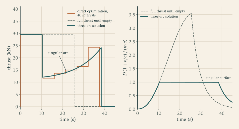
Two kinds of method. The two examples illustrate the two families of numerical optimal control. An indirect method solves the boundary-value problem of the necessary conditions; Example 10.3 is its simplest form, in which the structure was known and only the switching events had to be found. A direct method discretizes the control and hands a finite-dimensional problem to an optimizer, as in Example 10.4. Indirect methods are accurate and need a good guess of the structure. Direct methods need no guess and return answers blurred by the grid. A published treatment of a Goddard problem uses both and finds that they agree (control-toolbox tutorial; see sources). Used together, each covers the other’s weakness.
10.6 The reference launcher is nowhere near its surface
Does the reference launcher, climbing at full thrust through maximum dynamic pressure, belong on a singular arc? Proposition 10.2 was derived for vertical flight, and the launcher is by then on a path inclined at about \(51^\circ\) , so the comparison is indicative, not exact. It is also not close.
Example 10.5: The launcher’s distance from the singular surface
Flight condition. At \(t=78.5\ \mathrm s\) on the reference ascent of Example 7.6, the instant of maximum dynamic pressure, the integration gives \(z=14.40\ \mathrm{km}\) , \(v=542.0\ \mathrm{m/s}\) , and a mass of \(114.1\ \mathrm t\) . The dynamic pressure is \(32.83\ \mathrm{kPa}\) , so \(D=(32\,832)(0.3)(7.07)=69.64\ \mathrm{kN}\) . The thrust at that altitude is \(2461.6\ \mathrm{kN}\) , so \(c=F/\dot m_1=3035\ \mathrm{m/s}\) , and \(g=9.754\ \mathrm{m/s^2}\) .
The ratio.
Along the whole first-stage burn the ratio never exceeds \(0.078\) , reached near \(90\ \mathrm s\) . The launcher is more than a factor of twelve short of the surface. Put as a speed: at this altitude and mass the surface speed is \(1730\ \mathrm{m/s}\) , more than three times what the vehicle is doing.
Why so far. The surface speed is set by the mass carried per unit of drag area, the ballistic coefficient \(\beta=m/(C_DS)\) , which Chapter 12 will meet again. For the launcher at this instant \(\beta=114\,143/2.121=53\,800\ \mathrm{kg/m^2}\) ; for the sounding rocket at liftoff it is \(23\,600\ \mathrm{kg/m^2}\) . And the launcher accelerates gently: its thrust is \(1.3\) times its weight at liftoff against the sounding rocket’s \(6\) . A heavy, slowly accelerating vehicle is out of the dense air before it is fast enough for drag to matter. Drag is \(6\) percent of its weight at the worst instant.
A throttle bucket, priced. The same conclusion can be tested on the real trajectory. Run the first stage at \(70\) percent thrust and flow from \(65\) to \(90\ \mathrm s\) , extend the burn by \(7.5\ \mathrm s\) so that the same propellant is used, and solve Chapter 7’s three unknowns again for the \(200\ \mathrm{km}\) orbit. The result is \(\chi=1.609^\circ\) , \(\alpha_2=2.552^\circ\) , and an ideal velocity to orbit of \(9392.4\ \mathrm{m/s}\) , which is \(84.9\ \mathrm{m/s}\) more than the \(9307.6\ \mathrm{m/s}\) of Example 7.6. Maximum dynamic pressure falls from \(32.8\) to \(28.1\ \mathrm{kPa}\) . Throttling down in the atmosphere costs this vehicle velocity. If it is done, it is done to relieve the structure, and the price is now known.
For the launcher, then, the evidence on the chapter’s first question points one way. The condition of Proposition 10.2, which was derived for vertical flight, puts the surface at three times the vehicle’s speed, and the one throttle schedule tried on the curved ascent cost \(85\ \mathrm{m/s}\) . Neither is a proof of optimality for the real trajectory. Together they say that full thrust through the atmosphere is the right policy for performance, and that the singular arc belongs to small, hard-accelerating rockets.
10.7 Where to point in vacuum
Above the atmosphere the thrust magnitude is no longer in question; the engine runs at its one setting. What remains is the direction.
The system. A vehicle moves in a vertical plane above a flat, airless ground. Its state is downrange distance \(x\) , altitude \(z\) , the velocity components \(v_x\) and \(v_z\) , and mass \(m\) . Its control is the pitch \(\vartheta\) of the thrust, the angle of the thrust above the horizontal.
Assumptions. (i) The ground is flat and gravity is uniform, of magnitude \(g\) , straight down. (ii) There is no atmosphere. (iii) The engine runs at constant thrust \(F\) and constant flow \(F/c\) until cutoff. (iv) The altitude and both velocity components are prescribed at cutoff; the downrange distance is free. (v) The pitch may be chosen freely and changed instantly.
The equations are
and the payoff is the mass at cutoff, \(m(t_f)\) , which with constant flow is the same as asking for the earliest cutoff.
Costates. With \(p_x\) , \(p_z\) , \(p_{vx}\) , \(p_{vz}\) , and \(p_m\) paired with the five states,
Neither \(x\) nor \(z\) appears in \(\mathcal H\) , so \(\dot p_x=0\) and \(\dot p_z=0\) : both are constants. Downrange distance is free at cutoff, so \(p_x(t_f)=0\) , and therefore \(p_x\) is zero throughout. The velocity costates obey \(\dot p_{vx}=-p_x=0\) and \(\dot p_{vz}=-p_z\) . So \(p_{vx}\) is a constant and \(p_{vz}\) is a linear function of time:
The pointing condition. The pitch enters \(\mathcal H\) only through \(p_{vx}\cos\vartheta+p_{vz}\sin\vartheta\) , which is the dot product of the vector \((p_{vx},p_{vz})\) with the unit vector along the thrust. A dot product with a unit vector is largest when the unit vector points along the other one. Condition (ii) of Theorem 10.1 therefore says: point the thrust along the velocity costate. In terms of the angle, with \(p_{vx}\) positive,
Proposition 10.3 (linear-tangent steering law). Under assumptions (i) to (v), the pitch of the thrust along an optimal trajectory satisfies
where \(\vartheta_0\) is the initial pitch and \(p_z/p_{vx}\) is a constant with the units of inverse seconds.
The law has two constants, and with the cutoff time that makes three unknowns for the three terminal conditions of assumption (iv). The optimal control has been reduced to a root-finding problem in three numbers. Finding them is shooting on the costates: the two constants are the initial costate ratios \(p_{vz}(0)/p_{vx}\) and \(p_z/p_{vx}\) .
Why this shape. The thrust direction is the direction in which velocity is currently most valuable. A metre per second of vertical velocity acquired early lifts the vehicle for the whole remaining burn, so early in the burn vertical velocity carries the extra worth of the altitude it will buy; that extra worth, \(p_z\) per second remaining, shrinks linearly as the time left runs out. The pitch starts high and comes down. If altitude is not prescribed, \(p_z=0\) and the pitch is constant. If downrange distance is prescribed as well, \(p_x\) is no longer zero, \(p_{vx}\) becomes linear in time too, and the law is a ratio of two linear functions, the bilinear-tangent law (Exercise 12).
The same law is derived in a published set of lecture notes by the classical calculus of variations, with the remark that it formed the basis of the guidance mode used by the Saturn launch vehicles to reach a parking orbit (MIT 16.346 notes, Lecture 32; see sources).
Common mistake. Steering along the velocity in vacuum “to avoid steering loss”. The gravity turn did so in the atmosphere, for the structure’s sake. In vacuum the steering loss is one of two losses, and the optimum trades a little more of it for a larger saving in gravity loss. Section 10.8 measures the trade.
Example 10.6: Three constants for a flat, airless world
Setup. Take \(g=1.62\ \mathrm{m/s^2}\) , the Moon’s surface gravity (NASA Moon Fact Sheet; see sources), and a vehicle whose thrust acceleration \(F/m\) is held constant at \(4.0\ \mathrm{m/s^2}\) (illustrative; a real engine at constant thrust would accelerate harder as it lightened, and the law would be unchanged). It starts at rest on the ground and must arrive at \(z=20\ \mathrm{km}\) moving horizontally at \(v_x=1650\ \mathrm{m/s}\) (illustrative targets). Find \(\vartheta_0\) , \(p_z/p_{vx}\) , and \(t_f\) .
Closed forms. Within this example write \(\vartheta_f=\vartheta(t_f)\) for the pitch at cutoff, and abbreviate the rate \(p_z/p_{vx}\) as \(\varrho\) , so \(\tan\vartheta_f=\tan\vartheta_0-\varrho\,t_f\) . With \(\cos\vartheta=1/\sqrt{1+\tan^2\vartheta}\) and \(\sin\vartheta=\tan\vartheta/\sqrt{1+\tan^2\vartheta}\) , the velocity integrals are elementary:
The altitude is \(\int_0^{t_f}(t_f-t)\,\dot v_z\,\mathrm dt\) , which also has a closed form in the same functions.
Shooting. Three equations, \(v_x(t_f)=1650\ \mathrm{m/s}\) , \(v_z(t_f)=0\) , and \(z(t_f)=20\ \mathrm{km}\) , in three unknowns. Newton iteration from a rough guess converges to
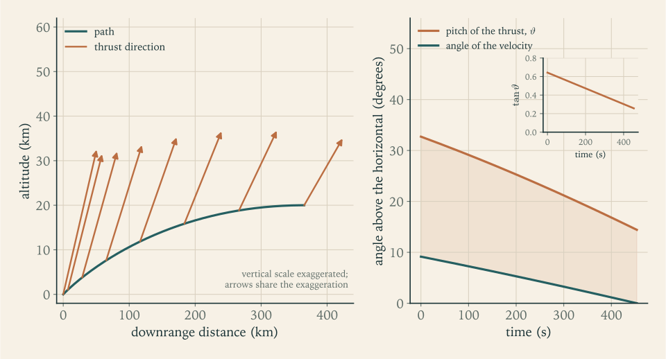
The pitch ends at \(\tan\vartheta=0.6424-(8.496\times10^{-4})(453.47)=0.2571\) , that is \(14.42^\circ\) . Figure 10.2 shows the path and the thrust direction along it.
Check. Substituting back: \(\sinh^{-1}0.6424=0.6048\) and \(\sinh^{-1}0.2571=0.2543\) , so \(v_x=(4.0/8.496\times10^{-4})(0.3505)=1650\ \mathrm{m/s}\) , to the four figures carried. An independent Runge-Kutta integration of the five equations of motion with this pitch history returns \(z=20.000\ \mathrm{km}\) , \(v_x=1650.0\ \mathrm{m/s}\) , \(v_z=0.0\ \mathrm{m/s}\) , and a downrange distance of \(365.3\ \mathrm{km}\) .
The cost. The engine supplies \((4.0)(453.47)=1813.9\ \mathrm{m/s}\) of ideal velocity to produce \(1650\ \mathrm{m/s}\) : a loss of \(163.9\ \mathrm{m/s}\) , the sum of gravity and steering losses. For comparison, the cheapest conceivable delivery of that speed and height is the energy bound \(\sqrt{1650^2+2(1.62)(20\,000)}=1669.5\ \mathrm{m/s}\) , which only an impulse at the ground could approach.
Validity. On this flat world nothing but the thrust opposes gravity, and the thrust does not do so for the whole burn. Its vertical component exceeds the weight only while the pitch is above \(\sin^{-1}(1.62/4.0)=23.9^\circ\) , which lasts until \(234.8\ \mathrm s\) . By then the vehicle is climbing at \(66\ \mathrm{m/s}\) , and for the second half of the burn it is being slowed in its climb, arriving level at the target height. The final pitch stays well above zero here because the target is low; with a target of \(50\ \mathrm{km}\) (Exercise 15) the law starts steeper and ends almost flat. Over a round body, the term \(v^2/r\) of Section 7.3 takes over part of the job as speed builds, and the pitch can fall through zero. A downrange distance of \(365\ \mathrm{km}\) is a fifth of the Moon’s radius, so for a real ascent the flat model would be a poor one; the example shows the method, not a lunar trajectory.
10.8 The law on a round Earth
The reference launcher’s second stage does not fly over a flat Earth with uniform gravity. Gravity turns with the local vertical and weakens with height, the costate equations are no longer so simple, and the law of Proposition 10.3 is not exactly optimal. It can still be used as a family of pitch programs with two constants, the pitch being measured from the local horizontal, and tested against the true optimum afterward.
There is now one more free parameter than there are conditions. The pitch-over angle \(\chi\) shapes the first stage’s gravity turn and so chooses the state at staging; the two tangent-law constants and the cutoff time then meet the three orbit conditions from that state. For each \(\chi\) there is one flight that reaches the orbit, and \(\chi\) can be chosen to make its ideal velocity least. Chapter 7’s family had no such freedom.
Example 10.7: The second stage steered by the tangent law
Setup. Revision A on a non-rotating Earth with the models and step counts of Example 7.6, so that the comparison is with that example. Stage 1 flies a gravity turn from a pitch-over of \(\chi\) at \(20\ \mathrm s\) . Stage 2 flies \(\tan\vartheta(t)=\tan\vartheta_0-(p_z/p_{vx})(t-t_{b,1})\) , with \(\vartheta\) measured from the local horizontal, and the three numbers \(\tan\vartheta_0\) , \(p_z/p_{vx}\) , and the burn time are found by Newton iteration so that the cutoff is at \(200\ \mathrm{km}\) , level, at \(7784.3\ \mathrm{m/s}\) .
One flight for each pitch-over angle.
| \(\chi\) | Initial pitch \(\vartheta_0\) | Gravity loss | Drag loss | Steering loss | Ideal velocity to orbit | Propellant left |
|---|---|---|---|---|---|---|
| \(2.0^\circ\) | \(9.1^\circ\) | \(1498.2\ \mathrm{m/s}\) | \(46.0\ \mathrm{m/s}\) | \(13.0\ \mathrm{m/s}\) | \(9341.4\ \mathrm{m/s}\) | \(405\ \mathrm{kg}\) |
| \(2.1^\circ\) | \(16.9^\circ\) | \(1468.6\ \mathrm{m/s}\) | \(48.9\ \mathrm{m/s}\) | \(5.1\ \mathrm{m/s}\) | \(9306.9\ \mathrm{m/s}\) | \(482\ \mathrm{kg}\) |
| \(2.2^\circ\) | \(24.7^\circ\) | \(1440.4\ \mathrm{m/s}\) | \(52.6\ \mathrm{m/s}\) | \(19.0\ \mathrm{m/s}\) | \(9296.3\ \mathrm{m/s}\) | \(505\ \mathrm{kg}\) |
| \(2.3^\circ\) | \(32.1^\circ\) | \(1413.5\ \mathrm{m/s}\) | \(57.0\ \mathrm{m/s}\) | \(55.5\ \mathrm{m/s}\) | \(9310.3\ \mathrm{m/s}\) | \(473\ \mathrm{kg}\) |
| \(2.4^\circ\) | \(39.2^\circ\) | \(1387.6\ \mathrm{m/s}\) | \(62.7\ \mathrm{m/s}\) | \(115.4\ \mathrm{m/s}\) | \(9349.9\ \mathrm{m/s}\) | \(383\ \mathrm{kg}\) |
Reading the table. A larger pitch-over flattens the first stage’s path. Gravity loss falls steadily, by about \(28\ \mathrm{m/s}\) per tenth of a degree. But the flatter path leaves the second stage lower and with less upward velocity, so it must begin pitched further above its velocity, and the steering loss, small near \(2.1^\circ\) , climbs faster and faster. The total has a minimum between.
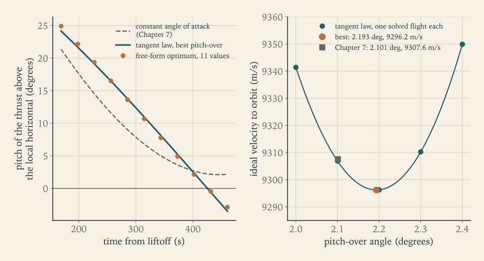
The best angle. A parabola through the three rows at \(2.1^\circ\) , \(2.2^\circ\) , and \(2.3^\circ\) has its vertex at \(\chi=2.193^\circ\) , and the flight solved at that angle has
an ideal velocity of \(9296.2\ \mathrm{m/s}\) , and \(505\ \mathrm{kg}\) of propellant unburned. The pitch ends at \(-3.5^\circ\) : for the last half minute the thrust points slightly below the horizon, holding down a vehicle that is by then nearly in orbit and would otherwise rise above its target. Staging occurs at \(75.0\ \mathrm{km}\) and \(3259.7\ \mathrm{m/s}\) with the path inclined at \(17.3^\circ\) , so the thrust jumps \(6.8^\circ\) above the velocity as the second stage lights.
Against Chapter 7.
| Quantity | Constant angle of attack (Example 7.6) | Tangent law, best \(\chi\) |
|---|---|---|
| Pitch-over angle | \(2.101^\circ\) | \(2.193^\circ\) |
| Gravity loss | \(1470.8\ \mathrm{m/s}\) | \(1442.3\ \mathrm{m/s}\) |
| Drag loss | \(49.0\ \mathrm{m/s}\) | \(52.3\ \mathrm{m/s}\) |
| Steering loss | \(3.5\ \mathrm{m/s}\) | \(17.4\ \mathrm{m/s}\) |
| Ideal velocity to orbit | \(9307.6\ \mathrm{m/s}\) | \(9296.2\ \mathrm{m/s}\) |
| Propellant left at cutoff | \(480\ \mathrm{kg}\) | \(505\ \mathrm{kg}\) |
The saving is \(11.3\ \mathrm{m/s}\) , and its composition is the lesson. The steering loss went up fivefold and the drag loss went up too; the gravity loss came down by more than both. Notice also what the tangent law does at Chapter 7’s own pitch-over angle: solved at \(\chi=2.101^\circ\) it needs \(9306.7\ \mathrm{m/s}\) , a saving of only \(0.9\ \mathrm{m/s}\) over the constant angle. Nearly all of the gain comes from being free to choose the pitch-over angle with the steering law, and very little from the shape of the law. Counting the pitch-over impulse of Section 7.7, which the larger angle raises from \(2.6\) to \(2.8\ \mathrm{m/s}\) , the saving is \(11.2\ \mathrm{m/s}\) .
What reaches the tanks. The ideal velocity is supplied by both stages, and the first stage’s share is not fixed: on the flatter path it spends longer in denser air, its thrust is a little lower, and the same propellant gives \(0.3\ \mathrm{m/s}\) less. The second stage therefore saves \(11.0\ \mathrm{m/s}\) and not \(11.3\) , and that is what the \(25\ \mathrm{kg}\) of extra propellant at cutoff is worth.
Is the tangent law itself optimal here? Test it as Example 10.4 tested the Goddard structure. Let the second stage’s pitch be an arbitrary piecewise-linear function of time through \(11\) equally spaced values, and minimize the ideal velocity over those \(11\) values, the pitch-over angle, and the burn time, subject to the three cutoff conditions, starting from the tangent-law flight. The optimizer lowers the ideal velocity by \(0.07\ \mathrm{m/s}\) , to \(9296.16\ \mathrm{m/s}\) , and the tangents of its pitch values, \(0.464\) , \(0.407\) , \(0.351\) , \(0.296\) , \(\dots\) , \(-0.050\) , lie within \(0.016\) of a straight line. On a round Earth the flat-Earth law is not exact, and the error is seven hundredths of a metre per second. Figure 10.3 shows the pitch histories.
10.9 What flying at zero angle of attack costs
The first stage was not included in that optimization. It flew a gravity turn, with the thrust along the velocity, and the reason given in Section 7.7 was structural: an angle of attack in dense air loads the vehicle sideways in proportion to \(q\,\alpha\) . A point mass has no structure, so the point-mass optimum would not respect that rule. How much is the rule costing?
Example 10.8: A degree of angle of attack, priced
Experiment. Let the first stage carry a small angle of attack \(\alpha_1\) , nose above the velocity, raised linearly from zero at \(30\ \mathrm s\) to its full value at \(40\ \mathrm s\) and held to staging. The second stage flies the tangent law, and the pitch-over angle is re-optimized for each \(\alpha_1\) . As in Chapter 7 the model has no aerodynamic lift, so the angle acts only by turning the thrust; at these angles the lift of a slender body would add to the turning force by roughly a fifth (Chapter 11 estimates it).
| \(\alpha_1\) | Best \(\chi\) | Ideal velocity to orbit | With pitch-over impulse | Saving | Peak \(q\) | \(q\,\alpha_1\) at the peak |
|---|---|---|---|---|---|---|
| \(0\) | \(2.193^\circ\) | \(9296.2\ \mathrm{m/s}\) | \(9299.0\ \mathrm{m/s}\) | \(33.6\ \mathrm{kPa}\) | \(0\) | |
| \(1^\circ\) | \(2.690^\circ\) | \(9281.8\ \mathrm{m/s}\) | \(9285.2\ \mathrm{m/s}\) | \(13.8\ \mathrm{m/s}\) | \(35.0\ \mathrm{kPa}\) | \(0.61\ \mathrm{kPa\cdot rad}\) |
| \(3^\circ\) | \(3.713^\circ\) | \(9256.8\ \mathrm{m/s}\) | \(9261.5\ \mathrm{m/s}\) | \(37.5\ \mathrm{m/s}\) | \(38.5\ \mathrm{kPa}\) | \(2.02\ \mathrm{kPa\cdot rad}\) |
Reading the table. The optimizer uses the angle of attack to hold the nose up while it tips the vehicle over harder at the start: the path flattens sooner, gravity loss falls, and the lifted nose keeps the vehicle from sinking. Each degree is worth about \(13\ \mathrm{m/s}\) . So the gravity turn is not the optimum of the point-mass problem. It is what that problem is left with when the first stage is held to \(q\,\alpha=0\) , and over the range in the table the constraint costs about \(0.15\) percent of the ideal velocity per degree. Pushed further, the same family gains less for each degree and stops gaining near \(8^\circ\) , where the saving is \(69\ \mathrm{m/s}\) .
Why the constraint is kept. Three degrees through maximum dynamic pressure is a load of \(2\ \mathrm{kPa\cdot rad}\) on every flight, by design. Chapter 11 will show that an ordinary wind produces angles of attack of that size without being asked, and the structure must survive the wind in any case. Flying the planned trajectory at zero angle of attack leaves the whole of the structure’s allowance for the disturbances that cannot be planned. The \(38\ \mathrm{m/s}\) is the price of that policy, about \(90\ \mathrm{kg}\) of payload at Example 2.6’s exchange ratio of \(2.37\ \mathrm{kg}\) per metre per second, and vehicles pay it. The gravity turn is near-optimal in this limited sense: within \(0.4\) percent of the \(3^\circ\) trajectory, and within three quarters of a percent of the best this family of ramped angles can do, and every one of those trajectories would need a stronger structure to fly. Other first-stage steering laws were not tried.
10.10 Guidance: solving the problem again from where the vehicle is
Everything so far has been planning. A plan is a control history, computed before flight from a model: a thrust level and a pitch angle for each instant. A vehicle that simply plays the history back is under open-loop control. If the engine underperforms, the open-loop vehicle points where the plan says at each second and arrives somewhere else.
Closed-loop guidance replaces the stored history by a stored problem. At intervals during flight the vehicle measures its state and its acceleration, solves the steering problem from that state to the target, and flies the opening portion of the solution until the next measurement. For the upper stage the problem is the one of Section 10.8 with the first stage already behind: three unknowns, the present value of \(\tan\vartheta\) , the rate \(p_z/p_{vx}\) , and the time to go \(t_{\mathrm{go}}\) , and three orbit conditions. It is small enough to solve many times a minute.
Two facts make the scheme sound. If nothing has gone wrong, re-solving changes nothing: the remainder of an optimal trajectory is itself optimal for the problem that starts from any state on it, which is the principle of optimality on which the cited course is built, so the new solution is the tail of the old one. And if something has gone wrong, the new solution is the best that can be done from where the vehicle actually is. Repeating an optimization from each measured state and applying only the first part of each answer is the method called model predictive control in Dynamic Programming and Optimal Control (math.dynamic-programming-and-optimal-control.approximate-dp-mpc), here with a horizon that shrinks to the cutoff. The published notes cited above describe the Saturn vehicles’ scheme in the same terms, as an iterated solution of the linear-tangent problem (MIT 16.346 notes, Lecture 32; see sources).
Guidance in this sense decides where the thrust should point. Making the vehicle point there is a different problem, with different mathematics, and it is the subject of Chapter 11.
Why the first stage is flown open-loop. In the atmosphere the steering is constrained by the structure, as Section 10.9 found, and an optimizer free to command angles of attack would command them. The usual division, which this course follows at the level of principle, is a pre-computed program of pitch against time through the dense air, optimized on the ground over a few parameters such as \(\chi\) , and closed-loop guidance once the dynamic pressure has become negligible.
Example 10.9: A thrust shortfall, with and without guidance
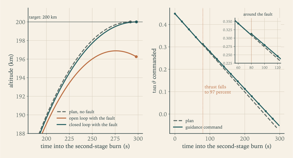
The fault. Fly the optimal plan of Example 10.7. At \(80\ \mathrm s\) into the second-stage burn the engine’s thrust and flow drop by \(3\) percent and stay there (an illustrative fault). The exhaust velocity is unchanged.
Open loop. The vehicle follows the planned pitch history. If it shuts down at the planned time, after \(291.60\ \mathrm s\) of burning, it is at \(196.6\ \mathrm{km}\) with a speed of \(7562.9\ \mathrm{m/s}\) , which is \(221\ \mathrm{m/s}\) short, on a path angled \(0.31^\circ\) downward. The two-body formulas of Chapter 8 give that state a perigee \(509\ \mathrm{km}\) below the surface: it is not in orbit. If instead it keeps to the planned pitch law and burns on until its speed reaches \(7784.3\ \mathrm{m/s}\) , which takes \(6.41\ \mathrm s\) more, it cuts off at \(196.3\ \mathrm{km}\) on a path angled \(0.42^\circ\) downward, in an orbit of \(144\) by \(241\ \mathrm{km}\) . That perigee is below the \(150\ \mathrm{km}\) working threshold of Section 8.7.
Closed loop. Every \(20\ \mathrm s\) (an illustrative cycle) the three unknowns are re-solved from the current state, using the thrust then measured. The first four solutions, before the fault, reproduce the plan: each returns the planned rate \(1.748\times10^{-3}\ \mathrm{s^{-1}}\) and a total burn of \(291.60\ \mathrm s\) , and the pitch tangent returned at \(20\ \mathrm s\) is \(0.4135\) , the plan’s own value \(0.44845-(0.0017480)(20)\) at that instant. The solution at \(80\ \mathrm s\) sees the reduced thrust:
| Burn time elapsed | \(\tan\vartheta\) now | Rate \(p_z/p_{vx}\) | Time to go | Predicted total burn |
|---|---|---|---|---|
| \(60\ \mathrm s\) | \(0.3436\) | \(1.748\times10^{-3}\ \mathrm{s^{-1}}\) | \(231.60\ \mathrm s\) | \(291.60\ \mathrm s\) |
| \(80\ \mathrm s\) | \(0.3127\) | \(1.667\times10^{-3}\ \mathrm{s^{-1}}\) | \(218.19\ \mathrm s\) | \(298.19\ \mathrm s\) |
| \(100\ \mathrm s\) | \(0.2794\) | \(1.667\times10^{-3}\ \mathrm{s^{-1}}\) | \(198.19\ \mathrm s\) | \(298.19\ \mathrm s\) |
| \(280\ \mathrm s\) | \(-0.0207\) | \(1.667\times10^{-3}\ \mathrm{s^{-1}}\) | \(18.19\ \mathrm s\) | \(298.19\ \mathrm s\) |
The plan called for \(\tan\vartheta=0.3086\) at \(80\ \mathrm s\) ; guidance raises it to \(0.3127\) , lifting the nose by \(0.21^\circ\) , lowers the rate, and extends the burn by \(6.59\ \mathrm s\) . Every later solution confirms the new plan. The vehicle cuts off after \(298.19\ \mathrm s\) at \(200.0\ \mathrm{km}\) , level, at \(7784.3\ \mathrm{m/s}\) : the target orbit. It has spent \(9298.0\ \mathrm{m/s}\) of ideal velocity, \(1.8\ \mathrm{m/s}\) more than planned, because the weaker engine fights gravity for longer, and it has \(501\ \mathrm{kg}\) of propellant left where the plan had \(505\) .
Reading the result. Guidance did not restore the thrust and could not have. It re-planned the path. The open-loop vehicle with the same engine and the same propellant ends in the ocean or in an orbit that decays; the guided one loses four kilograms of reserve. Figure 10.4 shows the three flights.
10.11 The reference launcher after optimization
Chapter 9 issued Revision B and flew it once, on the rotating ground and with the constant-angle law, as a test. The results of this chapter can be applied to that flight directly. With the tangent law on the second stage and the pitch-over angle chosen by the parabola of Example 10.7, Revision B reaches the \(200\ \mathrm{km}\) parking orbit as follows.
Example 10.10: Revision B, steered by the tangent law
Inputs. Revision B exactly as Example 9.8 built it: liftoff mass \(162\,985\ \mathrm{kg}\) , the engines and burn times listed there, launched due east from latitude \(28.5^\circ\) with the ground and the air moving as in that example. Nothing is changed but the steering.
| Quantity | Constant angle (Example 9.8) | Tangent law, best \(\chi\) |
|---|---|---|
| Pitch-over angle | \(2.357^\circ\) | \(2.470^\circ\) |
| Stage 2 steering | \(\alpha_2=0.180^\circ\) | \(\vartheta\) from \(22.9^\circ\) to \(-6.0^\circ\) , rate \(1.903\times10^{-3}\ \mathrm{s^{-1}}\) |
| Cutoff | \(447.8\ \mathrm s\) | \(447.3\ \mathrm s\) |
| Ideal velocity used to the parking orbit | \(8874.3\ \mathrm{m/s}\) | \(8858.7\ \mathrm{m/s}\) |
| Propellant unburned | \(951\ \mathrm{kg}\) | \(987\ \mathrm{kg}\) |
| Left after the transfer to \(400\ \mathrm{km}\) | \(317.1\ \mathrm{m/s}\) | \(332.2\ \mathrm{m/s}\) |
The optimized steering saves \(15.6\ \mathrm{m/s}\) of ideal velocity and leaves \(36\ \mathrm{kg}\) more propellant. As in Example 10.7 the first stage gives \(0.4\ \mathrm{m/s}\) less on the flatter path, so the capability in hand rises by \(15.1\ \mathrm{m/s}\) . After the transfer the model flight has \(332.2\ \mathrm{m/s}\) in hand against Chapter 9’s provision of \(291.7\ \mathrm{m/s}\) for allowance and reserve, where the constant-angle flight had \(317.1\ \mathrm{m/s}\) .
What that does and does not mean. The gain is real within the model, and it is small: a sixth of one percent of the budget. It is a statement about the model’s own lines. Chapter 9’s allowance for steering exists because real vehicles lose far more to steering than this idealized planar flight does, through winds, through constraints on the path, and through the limits on angle of attack that Section 10.9 priced. Optimal steering in the same idealized model does not touch any of those. It does change what the allowance is measured from. Chapter 9 set each of its two large items as the cited median less the model flight’s own loss, and the tangent-law flight has losses of its own: \(11.5\ \mathrm{m/s}\) of steering and \(59.1\ \mathrm{m/s}\) of drag, taken against the velocity relative to the ground. So the provision of \(291.7\ \mathrm{m/s}\) , which was computed for another flight, is not the right yardstick for this one, and the rise of the surplus over it from \(25\) to \(40\ \mathrm{m/s}\) should not be read as margin gained. The vehicle is not resized in this chapter. The \(15.6\ \mathrm{m/s}\) is recorded as what it is, a slightly better use of the same hardware, and Chapter 12 applies Chapter 9’s rule to the flight actually flown.
Direct ascent, revisited. Section 9.7 compared flight plans by the payload the Revision A stages could carry to \(400\ \mathrm{km}\) on a non-rotating Earth with nothing held back, and promised that better steering would narrow the gap between direct ascent and a parking orbit without closing it. With the tangent law and the best pitch-over angle for each plan, the parking-orbit route delivers \(5262\ \mathrm{kg}\) where the constant-angle law delivered \(5237\ \mathrm{kg}\) , and direct ascent delivers \(4320\ \mathrm{kg}\) where it delivered \(4208\ \mathrm{kg}\) . The direct profile gains more, because it was the one flown with large angles of attack, and the gap closes from \(1029\) to \(942\ \mathrm{kg}\) . It remains \(18\) percent of the payload. The preference for a parking orbit was never a consequence of crude steering.
The effect of this chapter on the reference launcher, collected:
| Item | Result |
|---|---|
| Thrust level in the atmosphere | full thrust is optimal; the launcher reaches at most \(0.078\) of the way to its singular surface |
| A throttle bucket to \(70\) percent from \(65\) to \(90\ \mathrm s\) | lowers peak dynamic pressure from \(32.8\) to \(28.1\ \mathrm{kPa}\) and costs \(84.9\ \mathrm{m/s}\) |
| Stage 1 steering | gravity turn kept; an angle of attack of \(1^\circ\) would save \(13.8\ \mathrm{m/s}\) at a design load of \(0.61\ \mathrm{kPa\cdot rad}\) |
| Stage 2 steering | tangent law; within \(0.07\ \mathrm{m/s}\) of the free-form optimum |
| Saving against Chapter 7’s law, Revision A, non-rotating | \(11.3\ \mathrm{m/s}\) |
| Saving on Revision B’s test flight | \(15.6\ \mathrm{m/s}\) ; left after the transfer \(332.2\ \mathrm{m/s}\) against a provision of \(291.7\ \mathrm{m/s}\) |
| Guidance | closed-loop on stage 2; absorbs a \(3\) percent thrust loss for \(1.8\ \mathrm{m/s}\) |
| Budget and masses | unchanged here: \(9306.3\ \mathrm{m/s}\) and Revision B; the saving is carried to Chapter 12 |
The large losses were never the steering law’s to remove. Of the \(1.5\ \mathrm{km/s}\) lost on the way to orbit, the best steering this model allows recovers about one percent. The gravity loss is set by how long the vehicle spends climbing steeply, and that is decided by its thrust-to-weight ratio and by the altitude it must reach before it can fly level, not by the fine shape of the pitch history.
Where this chapter’s model stops being accurate. The Goddard analysis assumed vertical flight and a constant drag coefficient; near the speed of sound the coefficient rises and the surface speed there would be lower than computed, though not by a factor of three. The steering results assume a point mass that can point its thrust anywhere at once. The tangent-law flight asks the vehicle to swing its thrust \(6.8^\circ\) away from the velocity at the instant of staging and then to rotate steadily, nose down, at about a tenth of a degree per second for five minutes. A real vehicle has a moment of inertia, an engine that can deflect only so far, and, in the air, a tendency to turn the wrong way by itself. Whether the reference launcher can follow these commands, and what holds it on course through maximum dynamic pressure, is the question for Chapter 11.
Exercises
-
Name the five ingredients of an optimal-control problem and identify each for the upper-stage steering problem of Section 10.7. Then explain why the reference ascent of Example 7.6, with its three parameters and three terminal conditions, involved no optimization, and say which additional freedom Example 10.7 used.
Hint
List state, control, dynamics, terminal conditions, and payoff, and for Section 10.7 name each: five states, one control (the pitch), five equations, three prescribed final values, and the final mass. For the second part, count: Example 7.6 had three unknowns and three conditions. Example 10.7 kept the three conditions and had four unknowns, \(\chi\) and three for the upper stage.
-
For the sounding rocket of Example 10.1 with no atmosphere and uniform gravity \(g_0\) , compute the burn time, burnout speed, burnout altitude, and highest point for thrust equal to \(2\) and to \(12\) times the liftoff weight. Show that the time of the highest point is \(c\ln\mathcal R/g_0\) for every thrust level, and evaluate the costate \(p_v\) at liftoff.
Solution
With \(\zeta=0.6\) , \(\mathcal R=2.5\) , and \(c=2500\ \mathrm{m/s}\) , Section 1.6 gives \(t_b=\zeta c/(\psi_0g_0)\) , \(v_b=c\ln\mathcal R-g_0t_b\) with \(c\ln\mathcal R=2290.7\ \mathrm{m/s}\) , and \(z_b=c[(\tau-t_b)\ln(1-t_b/\tau)+t_b]-\tfrac12g_0t_b^2\) with \(\tau=c/(\psi_0g_0)\) . The coast adds \(v_b^2/(2g_0)\) .
Thrust-to-weight ratio Burn time Burnout speed Burnout altitude Highest point \(2\) \(76.48\ \mathrm s\) \(1540.7\ \mathrm{m/s}\) \(45.72\ \mathrm{km}\) \(166.75\ \mathrm{km}\) \(12\) \(12.75\ \mathrm s\) \(2165.7\ \mathrm{m/s}\) \(11.60\ \mathrm{km}\) \(250.75\ \mathrm{km}\) Time of the highest point. After burnout the speed is \(v(t)=c\ln\mathcal R-g_0t\) , because gravity has removed \(g_0t\) since liftoff whether the engine was running or not. It vanishes at \(t_f=c\ln\mathcal R/g_0=2290.7/9.80665=233.6\ \mathrm s\) , with no reference to the thrust.
The costate. \(p_v=t_f-t\) , so \(p_v(0)=233.6\ \mathrm s\) : a metre per second of speed given to the vehicle at liftoff raises the highest point by \(233.6\ \mathrm m\) , since the vehicle keeps that extra speed for the whole flight.
-
Prove that in the Goddard problem without drag the switching function is strictly decreasing even when gravity varies with altitude as \(g(z)=\mu_E/(R_E+z)^2\) . Use the costate equations and the terminal condition on \(p_z\) to show first that \(p_z\ge1\) and \(p_v\ge0\) throughout the flight.
Solution
With \(D=0\) the costate equations are \(\dot p_z=p_v\,\mathrm dg/\mathrm dz\) , \(\dot p_v=-p_z\) , and \(\dot p_m=p_vF/m^2\) , with \(p_z(t_f)=1\) and \(p_v(t_f)=0\) . For inverse-square gravity \(\mathrm dg/\mathrm dz=-2g/r\) is negative.
Signs of the costates. Run time backward with \(s=t_f-t\) . Then \(\mathrm dp_v/\mathrm ds=p_z\) and \(\mathrm dp_z/\mathrm ds=(2g/r)\,p_v\) , starting from \(p_v=0\) and \(p_z=1\) . Let \(s^\ast\) be the largest value such that \(p_z\ge1\) on \([0,s^\ast]\) . On that interval \(p_v\) is the integral of a positive function, so \(p_v\ge0\) , hence \(\mathrm dp_z/\mathrm ds\ge0\) and \(p_z\) does not decrease. If \(s^\ast\) were less than \(t_f\) , continuity would give \(p_z\) positive on a slightly longer interval, where the same argument shows \(p_v\ge0\) and \(p_z\) nondecreasing, so \(p_z\ge1\) there too, contradicting the choice of \(s^\ast\) . Therefore \(p_z\ge1\) and \(p_v\ge0\) on the whole flight.
The switching function. Exactly as in Example 10.1,
\[ \frac{\mathrm d\mathcal H_F}{\mathrm dt}=\frac{\dot p_v}{m}+\frac{p_vF}{cm^2}-\frac{\dot p_m}{c}=-\frac{p_z}{m}\le-\frac1m , \]which is strictly negative. The switching function crosses zero at most once, downward, and cannot remain at zero, so the only candidate is full thrust followed by a coast. Variable gravity changes the prices, since \(p_z\) now exceeds \(1\) early in the flight, but not the structure.
-
Starting from the Hamiltonian of Section 10.3, derive the three costate equations, state the units of each costate when the payoff is an altitude in metres, and state the three terminal conditions with the reason for each. Then explain in one or two sentences what \(p_m(t)\) measures.
Hint
Compute \(-\partial\mathcal H/\partial z\) , \(-\partial\mathcal H/\partial v\) , and \(-\partial\mathcal H/\partial m\) term by term; only \(D\) and \(g\) depend on \(z\) , only \(D\) and the first term on \(v\) . Units are metres divided by the unit of the state. For the terminal conditions use (iii) of Theorem 10.1 with altitude as payoff, speed free, mass prescribed. The costate \(p_m\) is the height gained per kilogram of extra mass in hand at time \(t\) .
-
Suppose the drag law is \(D=k(z)\,v^{n}\) for a constant exponent \(n\) . (a) Show from Proposition 10.2 that the singular surface is \(D\,(n-1+v/c)=mg\) . (b) For \(n=1\) , which describes very slow flight through a viscous fluid, show that the surface speed satisfies \(k\,v^2=mgc\) and interpret the fact that no speed is “too fast” when \(c\) is infinite. (c) For \(n=2\) recover the result of the text.
Solution
(a) For \(D=k(z)v^n\) , \(v\,\partial D/\partial v=nD\) . Substituting in Proposition 10.2,
\[ nD+\frac vc\,D-D-mg=0\qquad\Longrightarrow\qquad D\Bigl(n-1+\frac vc\Bigr)=mg . \](b) With \(n=1\) this is \(Dv/c=mg\) , and \(D=kv\) gives \(kv^2=mgc\) , so the surface speed is \(\sqrt{mgc/k}\) . It grows without bound as \(c\to\infty\) . The reason is that linear drag removes momentum at the rate \(kv\) per second, which is \(k\) per metre climbed, the same at every speed. Climbing faster costs nothing extra in drag for a given height and saves gravity loss, so without the mass penalty there would be no reason ever to slow down. The finite exhaust velocity supplies the only restraint: momentum spent against drag is bought with propellant.
(c) With \(n=2\) the factor is \(1+v/c\) , the result of the text. For any \(n\) above \(1\) the surface exists even for infinite \(c\) , at \(D=mg/(n-1)\) .
-
For the sounding rocket of Example 10.2 at \(z=8\ \mathrm{km}\) and \(m=350\ \mathrm{kg}\) , compute the air density, the terminal velocity, and the speed on the singular surface, solving the cubic by a method of your choice and stating how you checked the root. By what percentage does the factor \(1+v/c\) lower the speed?
Solution
At \(8\ \mathrm{km}\) , \(\rho=(1.217)\exp(-8/8.5)=0.4748\ \mathrm{kg/m^3}\) and \(g=9.7737\ \mathrm{m/s^2}\) , so \(\tfrac12\rho C_DS=\tfrac12(0.4748)(0.02121)=0.005036\ \mathrm{kg/m}\) and \(mg=(350)(9.7737)=3420.8\ \mathrm N\) .
Terminal velocity. \(\sqrt{3420.8/0.005036}=824.2\ \mathrm{m/s}\) .
Singular surface. The cubic \(0.005036\,v^2(1+v/2500)=3420.8\) has a left side that increases with \(v\) , is below the right side at \(v=0\) , and is above it at \(v=824.2\ \mathrm{m/s}\) , so bisection on that bracket converges to the single positive root,
\[ v=725.6\ \mathrm{m/s}. \]Check: \((0.005036)(725.6)^2(1+0.2902)=3421\ \mathrm N\) . The factor \(1+v/c\) lowers the speed by \(12.0\) percent. The reduction grows with altitude, because the surface speed itself grows and with it the ratio \(v/c\) .
-
A student writes: “The Hamiltonian of the Goddard problem is linear in \(F\) , so by the maximum principle the optimal thrust is always \(F_{\max}\) or \(0\) . The rocket should therefore burn at full thrust until empty, with or without air.” (a) State exactly which step fails. (b) Use the numbers of Example 10.3 to show how much height the student’s flight loses. (c) Name the calculation that would have revealed the gap in the argument.
Solution
(a) The step from “linear in \(F\) ” to “always on a bound” fails. The maximum condition selects \(F_{\max}\) where \(\mathcal H_F\) is positive and \(0\) where it is negative, and is silent where \(\mathcal H_F=0\) . If \(\mathcal H_F\) vanishes on an interval, any thrust satisfies the condition there and the control must be found from the requirement that \(\mathcal H_F\) stay zero.
(b) In Example 10.3 the full-thrust flight reaches \(166.90\ \mathrm{km}\) and the three-arc flight \(174.95\ \mathrm{km}\) . The student’s rocket loses \(8.05\ \mathrm{km}\) , nearly five percent, with the same propellant.
(c) Differentiating the switching function along the trajectory. Without drag the derivative is \(-p_z/m\) , strictly negative, and the student’s conclusion holds. With drag it is \(-p_z/m+(p_v/m^2)(\partial D/\partial v+D/c)\) , which has no fixed sign, so the function can dwell at zero.
-
On a singular arc with quadratic drag, show that the drag equals the weight divided by \(1+v/c\) , so that drag is always less than weight on the arc. Evaluate \(D/(mg)\) at the start and at the end of the arc in Example 10.3, and explain why the vehicle nevertheless needs more thrust at the end than at the start.
Solution
On the arc \(D(1+v/c)=mg\) , so \(D=mg/(1+v/c)\) , which is less than \(mg\) for every positive speed.
At the start of the arc in Example 10.3, \(v=571.8\ \mathrm{m/s}\) and \(D/(mg)=1/(1+0.2287)=0.814\) . At the end, \(v=1689.5\ \mathrm{m/s}\) and \(D/(mg)=1/(1+0.6758)=0.597\) .
The thrust must supply drag, weight, and the acceleration needed to stay on the surface: \(F=D+mg+m\dot v\) . At the start, \(D=3009\ \mathrm N\) and \(mg=3697\ \mathrm N\) , so of the \(12\,070\ \mathrm N\) of thrust \(5364\ \mathrm N\) accelerates the vehicle, at \(14.2\ \mathrm{m/s^2}\) . At the end, \(D=1159\ \mathrm N\) and \(mg=1942\ \mathrm N\) , and \(21\,074\ \mathrm N\) of the \(24\,175\ \mathrm N\) goes to acceleration, \(105\ \mathrm{m/s^2}\) . Drag and weight have both fallen. What has grown is the rate at which the surface speed rises: it scales as \(\exp(z/2H)\) , so its relative growth rate is about \(v/(2H)\) , and that is three times larger at \(1690\ \mathrm{m/s}\) than at \(572\ \mathrm{m/s}\) , acting on a speed three times larger.
-
(Computation.) Write a program that flies the three-arc solution of Example 10.3 for the sounding rocket: full thrust to the surface, the feedback thrust of Section 10.4, then a coast, with each event located inside its step. Reproduce the highest point of \(174.95\ \mathrm{km}\) , and tabulate the highest point of the three-arc flight and of the full-thrust flight for maximum thrust equal to \(3\) , \(4\) , \(6\) , and \(10\) times the liftoff weight. Between which two values does the singular arc first appear?
Answer
Highest points, three-arc construction and full thrust: at \(3\) times liftoff weight, \(164.35\) and \(164.35\ \mathrm{km}\) (the surface is never reached); at \(4\) , \(170.42\) and \(169.61\ \mathrm{km}\) ; at \(6\) , \(174.95\) and \(166.90\ \mathrm{km}\) ; at \(10\) , \(177.94\) and \(153.72\ \mathrm{km}\) . The arc first appears between \(3\) and \(4\) .
A closer look at that interval needs one more degree of freedom than the construction has. Fly full thrust to the surface, follow the surface until a chosen time, then full thrust until the tanks are empty, then coast, and maximize the height over the time of leaving. The construction of Example 10.3 is the member of this family that stays on the surface as long as it can, and full thrust throughout is the member that leaves at once. Four regimes appear. Below \(3.198\) times liftoff weight the surface is not reached. From \(3.198\) to \(3.297\) it is crossed, and the best flight is still full thrust throughout. From \(3.297\) to \(4.89\) the best flight has four arcs: it leaves the surface before the feedback thrust has risen to \(F_{\max}\) . Above \(4.89\) the feedback thrust never reaches \(F_{\max}\) and the three arcs are optimal.
Maximum thrust over liftoff weight Best height On the surface Full thrust is lower by Riding the surface to saturation is lower by \(3.3\) \(166.8852\ \mathrm{km}\) \(29.35\) to \(29.48\ \mathrm s\) \(0.02\ \mathrm m\) \(12\ \mathrm m\) \(3.4\) \(167.529\ \mathrm{km}\) \(26.92\) to \(30.40\ \mathrm s\) \(18\ \mathrm m\) \(9\ \mathrm m\) \(4\) \(170.4233\ \mathrm{km}\) \(19.22\) to \(34.98\ \mathrm s\) \(810\ \mathrm m\) \(0.6\ \mathrm m\) At \(4\) the construction stays on the surface until its thrust saturates at \(37.47\ \mathrm s\) , two and a half seconds after the best flight has left. None of this changes the exercise’s table at its printed precision. It does change the reading of Proposition 10.2: the surface is where a singular arc must lie, and when to join it and when to leave it are separate questions, settled here by computing the family.
-
(Computation.) Repeat the direct transcription of Example 10.4 with \(20\) intervals instead of \(40\) . Report the final time, the highest point, and the thrust fractions, and explain why the height is lower than with \(40\) intervals and why neither can exceed the three-arc value.
Answer
With \(20\) intervals of \(10.65\ \mathrm s\) the optimizer returns \(t_f=213.0\ \mathrm s\) and thrust fractions \(1.00\) , \(0.38\) , \(0.59\) , \(0.42\) , then zero. The altitude at that time is \(174.67\ \mathrm{km}\) , and the vehicle is still climbing there at \(20.7\ \mathrm{m/s}\) ; coasting on, that thrust history tops out \(2.2\ \mathrm s\) later at \(174.70\ \mathrm{km}\) , which is the figure to compare. (On this grid the final time also sets the length of every burn interval, so the optimizer gives up the last \(23\ \mathrm m\) of coast for better-placed switches.) The coarser grid is a more restricted family of controls, so its best height is lower than the \(174.94\ \mathrm{km}\) of \(40\) intervals, and both are restrictions of the continuous problem, whose optimum is \(174.95\ \mathrm{km}\) .
-
This exercise uses Chapter 7. At the flight condition of Example 7.2 the reference launcher is at \(z=12\ \mathrm{km}\) and \(v=450\ \mathrm{m/s}\) with mass \(121\,035\ \mathrm{kg}\) , drag \(63.7\ \mathrm{kN}\) , weight \(1181.5\ \mathrm{kN}\) , and thrust \(2447\ \mathrm{kN}\) at a flow of \(811.1\ \mathrm{kg/s}\) . (a) Compute the ratio \(D(1+v/c)/(mg)\) . (b) By what factor would the product \(C_DS\) have to grow for the launcher to be on its singular surface there? (c) Explain, using the scaling of \(S/m\) with vehicle size from Section 7.6, why small launchers are closer to the surface than large ones.
Solution
(a) \(c=F/\dot m=2.447\times10^{6}/811.1=3016.9\ \mathrm{m/s}\) , so
\[ \frac{D(1+v/c)}{mg}=\frac{(63.7)(1+450/3016.9)}{1181.5}=\frac{73.2}{1181.5}=0.0620 . \](b) The ratio is proportional to \(C_DS\) at fixed speed, altitude, and mass, so \(C_DS\) would have to grow by \(1/0.0620=16.1\) times.
(c) The ratio is \(D(1+v/c)/(mg)\) and \(D/m\) is proportional to \(C_DS/m\) . For geometrically similar vehicles \(S/m\) scales as \(m^{-1/3}\) , so on the same trajectory a vehicle of one thousandth the mass has a ratio ten times larger, and its surface speed, which goes as the square root of \(m/(C_DS)\) , is lower by \(1000^{1/6}=3.2\) . That factor is about the gap between the reference launcher’s speed and its surface speed in Example 10.5. A launcher of a few hundred kilograms flying this trajectory would be near its singular surface; one of \(150\ \mathrm t\) is not. Small rockets also tend to accelerate harder, which moves them closer still.
-
In the flat-Earth steering problem of Section 10.7, suppose the downrange distance at cutoff is prescribed as well. (a) Which terminal condition of Theorem 10.1 changes, and what does it now say about \(p_x\) ? (b) Solve the costate equations and show that \(\tan\vartheta\) is a ratio of two linear functions of time. (c) Count unknowns and terminal conditions and confirm that they still match.
Solution
(a) With \(x(t_f)\) prescribed, condition (iii) no longer requires \(p_x(t_f)=0\) ; the costate \(p_x\) is unrestricted at the final time. It is still constant, because \(x\) does not appear in \(\mathcal H\) .
(b) The equations \(\dot p_{vx}=-p_x\) and \(\dot p_{vz}=-p_z\) now both have constant right sides, so
\[ p_{vx}(t)=p_{vx}(0)-p_x\,t,\qquad p_{vz}(t)=p_{vz}(0)-p_z\,t,\qquad \tan\vartheta(t)=\frac{p_{vz}(0)-p_z\,t}{p_{vx}(0)-p_x\,t}. \]The pointing condition is unchanged: thrust along \((p_{vx},p_{vz})\) .
(c) Only the direction of the costate vector matters for the pitch, so the four constants count as three ratios. With the cutoff time that makes four unknowns, and the terminal conditions are now four: \(x\) , \(z\) , \(v_x\) , and \(v_z\) . The count matches, as it did with three and three when \(x\) was free.
-
For constant thrust acceleration \(F/m\) and the law \(\tan\vartheta=\tan\vartheta_0-\varrho\,t\) , derive the closed form for \(v_x(t_f)\) quoted in Example 10.6 by taking \(\tan\vartheta\) as the variable of integration. Then evaluate \(v_z(t_f)\) from its closed form with the constants of that example and confirm that it vanishes to the accuracy of the printed figures.
Hint
Since \(\tan\vartheta=\tan\vartheta_0-\varrho\,t\) , \(\mathrm dt=-\mathrm d(\tan\vartheta)/\varrho\) , and \(\cos\vartheta=(1+\tan^2\vartheta)^{-1/2}\) , so \(v_x=(F/m)\varrho^{-1}\int(1+\tan^2\vartheta)^{-1/2}\,\mathrm d(\tan\vartheta)\) , taken from \(\tan\vartheta_f\) up to \(\tan\vartheta_0\) , and the antiderivative is \(\sinh^{-1}(\tan\vartheta)\) . For \(v_z\) the integrand is \(\tan\vartheta\,(1+\tan^2\vartheta)^{-1/2}\) with antiderivative \(\sqrt{1+\tan^2\vartheta}\) . With the printed constants the bracket is \(1.18856-1.03252\) and \(v_z\) comes out within a few hundredths of a metre per second of zero.
-
In the setting of Example 10.6, drop the altitude requirement: the vehicle must reach \(v_x=1650\ \mathrm{m/s}\) with \(v_z=0\) , at whatever height results. (a) Show that the optimal pitch is constant and equal to \(\sin^{-1}\bigl(g/(F/m)\bigr)\) . (b) Compute the pitch, the burn time, and the ideal velocity. (c) Find the altitude at cutoff and explain the answer. (d) Compare the burn time with that of Example 10.6 and say what the \(20\ \mathrm{km}\) of altitude cost.
Solution
(a) If altitude is free at cutoff, condition (iii) gives \(p_z(t_f)=0\) , and \(p_z\) is constant, so it is zero throughout. Then \(p_{vz}\) is constant as well as \(p_{vx}\) , and \(\tan\vartheta=p_{vz}/p_{vx}\) does not change. With a constant pitch and constant thrust acceleration the vertical acceleration \((F/m)\sin\vartheta-g\) is constant; starting from \(v_z=0\) and ending at \(v_z=0\) requires it to vanish. Hence \(\sin\vartheta=g/(F/m)\) .
(b) \(\sin\vartheta=1.62/4.0=0.405\) , so \(\vartheta=23.89^\circ\) . The horizontal acceleration is \(4.0\cos23.89^\circ=3.657\ \mathrm{m/s^2}\) , the burn lasts \(1650/3.657=451.16\ \mathrm s\) , and the ideal velocity is \((4.0)(451.16)=1804.6\ \mathrm{m/s}\) .
(c) The vertical velocity is zero throughout, so the altitude at cutoff is zero. The thrust’s vertical component exactly cancels the weight and the vehicle skims the ground. Nothing asked it to climb.
(d) Example 10.6 burns for \(453.47\ \mathrm s\) , which is \(2.31\ \mathrm s\) and \(9.2\ \mathrm{m/s}\) of ideal velocity more. Reaching \(20\ \mathrm{km}\) costs half a percent, because the law buys the altitude early, with a little extra pitch while the remaining burn is long.
-
(Computation.) Solve Example 10.6 again for a target altitude of \(50\ \mathrm{km}\) , by Newton iteration or a library root-finder on the three closed-form equations or on a numerical integration. Report \(\vartheta_0\) , the final pitch, \(p_z/p_{vx}\) , \(t_f\) , and the ideal velocity, and compare the loss with the \(163.9\ \mathrm{m/s}\) of the example.
Answer
\(\tan\vartheta_0=0.9627\) (\(\vartheta_0=43.91^\circ\) ), \(p_z/p_{vx}=2.061\times10^{-3}\ \mathrm{s^{-1}}\) , \(t_f=464.87\ \mathrm s\) , final pitch \(0.26^\circ\) , ideal velocity \(1859.5\ \mathrm{m/s}\) . The loss is \(209.5\ \mathrm{m/s}\) against \(163.9\ \mathrm{m/s}\) : the extra \(30\ \mathrm{km}\) cost \(45.6\ \mathrm{m/s}\) .
-
This exercise uses Chapter 2. From the table of Example 10.7: (a) pass a parabola through the ideal velocities at \(\chi=2.1^\circ\) , \(2.2^\circ\) , and \(2.3^\circ\) and find its vertex and minimum value; (b) estimate the ideal-velocity penalty of a pitch-over angle \(0.05^\circ\) away from the best; (c) convert that penalty to payload with the exchange ratio \(2.37\ \mathrm{kg}\) per metre per second of Example 2.6; (d) say what the flatness of the optimum implies about how accurately the pitch-over must be executed, and contrast this with the sensitivity of the pure gravity turn in Example 7.5.
Solution
(a) The three ideal velocities are \(9306.9\) , \(9296.3\) , and \(9310.3\ \mathrm{m/s}\) at spacing \(0.1^\circ\) . The second difference is \(9306.9-2(9296.3)+9310.3=24.6\ \mathrm{m/s}\) , so the parabola is \(9296.3+17.0\,(\chi-2.2)+1230\,(\chi-2.2)^2\) with \(\chi\) in degrees, the slope being \((9310.3-9306.9)/0.2=17.0\ \mathrm{m/s}\) per degree. Its vertex is at \(\chi=2.2-17.0/2460=2.193^\circ\) and its minimum is \(9296.3-17.0^2/4920=9296.2\ \mathrm{m/s}\) .
(b) A deviation of \(0.05^\circ\) costs \(1230\,(0.05)^2=3.1\ \mathrm{m/s}\) .
(c) \((3.1)(2.37)=7.3\ \mathrm{kg}\) of payload.
(d) Near an optimum the penalty is quadratic in the error, so a pitch-over executed to a twentieth of a degree loses a few kilograms. That is possible only because the upper stage’s steering absorbs the difference: for each \(\chi\) the tangent-law constants are re-solved and the orbit is still reached. In Example 7.5, where nothing downstream could compensate, half a degree of pitch-over separated a level burnout from a path \(10^\circ\) off level and about \(280\ \mathrm{km}\) too high. The gravity turn itself is as sensitive as before; closed-loop steering of the stage that follows removes the consequence.
-
A colleague objects to Example 10.7: “Your optimized flight has five times the steering loss of the Chapter 7 flight. It cannot be better.” (a) Using the two loss tables, show where the colleague’s accounting is incomplete. (b) Explain physically why thrust pitched above the velocity early in the second-stage burn reduces the gravity loss. (c) State what quantity should be compared between two flights that reach the same orbit, and why.
Solution
(a) Both flights end with the same speed, so by Proposition 7.2 their ideal velocities differ by the sum of the three loss differences. Steering is up by \(17.4-3.5=13.9\ \mathrm{m/s}\) and drag by \(52.3-49.0=3.3\ \mathrm{m/s}\) , but gravity is down by \(1470.8-1442.3=28.5\ \mathrm{m/s}\) . The net is \(-11.3\ \mathrm{m/s}\) . The colleague compared one line of a three-line account.
(b) At staging the vehicle is at less than half of orbital speed and its weight is mostly unsupported by the curvature term. Some force must hold the path up. If thrust is kept along the velocity, the only way to arrive level is to stage on a steeper path, so that the climb rate already banked carries the vehicle through, and a steeper first-stage path means more gravity loss on the first stage. Pitching the thrust above the velocity early in the second burn supports the vehicle directly, at a second-order cost in \(1-\cos\alpha\) , and lets the first stage fly flatter.
(c) The ideal velocity used, or equivalently the propellant left at cutoff. The individual losses are bookkeeping for where the ideal velocity went; only their sum is paid for in mass.
-
In Example 10.9 suppose the \(3\) percent loss of thrust and flow occurs at the start of the second-stage burn instead of at \(80\ \mathrm s\) . (a) Estimate the new burn time by assuming the ideal velocity needed is unchanged, and the propellant consumed. (b) Explain why the true ideal velocity needed is slightly larger and estimate the increase by scaling the \(1.8\ \mathrm{m/s}\) of the example. (c) The stage carries \(24\,881\ \mathrm{kg}\) ; is there enough? (d) If there were not, what should guidance aim for instead of the planned orbit, and why is “burn to depletion along the old plan” a poor answer?
Solution
(a) At \(97\) percent flow from the start, delivering the same ideal velocity means burning the same propellant, since \(c\) is unchanged, and that takes \(291.60/0.97=300.6\ \mathrm s\) . The propellant is \((83.60)(291.60)=24\,378\ \mathrm{kg}\) .
(b) The weaker engine spends longer below orbital speed, so the gravity loss grows. In the example the fault lasted \(218\ \mathrm s\) and cost \(1.8\ \mathrm{m/s}\) ; scaling by duration suggests about \(1.8\,(300.6/218.2)=2.5\ \mathrm{m/s}\) . A re-solution of the three unknowns with the reduced thrust from staging gives a burn of \(300.77\ \mathrm s\) and an ideal velocity higher by \(5.5\ \mathrm{m/s}\) : more than the scaling predicts, because the added seconds of fault fall early in the burn, where the path is steepest and gravity loss accrues fastest.
(c) The burn consumes \((0.97)(83.60)(300.77)=24\,389\ \mathrm{kg}\) of the \(24\,881\ \mathrm{kg}\) on board. There is enough, with \(493\ \mathrm{kg}\) to spare.
(d) Guidance should then aim for the best orbit the remaining propellant can reach: the same optimization with a different target, for example the highest perigee attainable, chosen so that the payload at least stays in orbit. Burning to depletion along the old plan steers for an orbit the vehicle can no longer reach and ends short of it at an arbitrary point, with the flight-path angle and altitude both wrong, as the open-loop flight of Example 10.9 did.
-
For each phase of the reference launcher’s flight, vertical rise, pitch-over and first-stage turn, second-stage burn, and the coast and transfer burns of Chapter 9, state whether open-loop or closed-loop steering is appropriate at the level of principle, and give the reason. Then compute the load \(q\,\alpha\) that would result if the second stage’s opening angle of attack of \(6.8^\circ\) were commanded at maximum dynamic pressure instead, and compare it with the largest entry in the table of Example 10.8.
Answer
Vertical rise and the first-stage turn: open-loop, a stored pitch program, because steering in dense air is limited by the load \(q\,\alpha\) and the program is designed around it. Second-stage burn: closed-loop, since the dynamic pressure is negligible and the steering problem is small enough to re-solve in flight. Coast and transfer burns: closed-loop in the same sense, each burn computed from the measured orbit. The load would be \((32.8\ \mathrm{kPa})(6.8^\circ)(\pi/180^\circ)=3.9\ \mathrm{kPa\cdot rad}\) , nearly twice the \(2.02\ \mathrm{kPa\cdot rad}\) of the last row of Example 10.8.
-
The first closed-loop solutions of Example 10.9 reproduced the plan. (a) Verify from the plan’s constants that the tangent of the planned pitch at \(60\ \mathrm s\) is the value in the table. (b) Give the argument, assuming the optimal trajectory from each state is unique, that a re-solution from a state on the optimal path must return the remainder of that path. (c) Explain why this property would fail if guidance minimized a different quantity at each re-solution, for example the time to go without regard to propellant.
Hint
(a) \(0.4484-(1.748\times10^{-3})(60)=0.3435\) , the table’s \(0.3436\) to the figures carried. (b) Suppose the re-solution from a point on the path found a different continuation. If it were better, splicing it onto the first part of the original path would beat the original, which was optimal; if it were only different and equally good, uniqueness is contradicted. (c) The argument needs the tail problem to have the same payoff as the original. A payoff that changes from one re-solution to the next makes each plan optimal for a different problem, and the pieces actually flown need not add up to an optimum of any of them.