The payload is in its orbit. The upper stage that put it there is beside it at \(400\ \mathrm{km}\) : two tonnes of aluminium tank, an engine, and about sixty kilograms of propellant kept back in Chapter 9 for one last burn. That burn lowers the perigee to \(50\ \mathrm{km}\) , and half an hour later the stage meets the atmosphere at \(7.9\ \mathrm{km/s}\) .
Each kilogram of it then carries \(31\ \mathrm{MJ}\) of kinetic energy. The propellant that put it there released \(9.7\ \mathrm{MJ}\) per kilogram when it burned. So the stage returns with three times the energy density of its own propellant, and every joule of it must go somewhere before the stage reaches the ground. Where it goes, how hard the stage decelerates, and how hot it gets are the first subject of this chapter. The analysis is one of the most economical in the field: a straight path, drag alone, an exponential atmosphere, and out comes a peak deceleration that does not depend on the body at all.
The second subject is the vehicle as a whole. Eleven chapters have each added or revised a piece of the reference launcher, in two revisions and a good many side calculations. The chapter’s second half runs the complete design loop one more time, to convergence, issues a final revision, traces every number in it to the chapter and the assumption it came from, and asks which of those assumptions would bring the design down first.
12.1 Thirty megajoules per kilogram
Example 12.1: The energy the upper stage brings back
The entry state. The disposal burn of Section 9.8 leaves the stage on an ellipse from \(400\ \mathrm{km}\) down to \(50\ \mathrm{km}\) . The vis-viva equation and the conservation of angular momentum (Chapter 8) give its state where it crosses \(120\ \mathrm{km}\) , a conventional height for the start of entry, used here as the entry interface:
The subscript on the speed is spelled out because \(v_e\) is the exhaust speed; the path angle is negative because the stage is descending. Both follow from the \(400\) by \(50\ \mathrm{km}\) ellipse alone, so they hold for every revision of the launcher.
Kinetic energy.
Against the propellant. Chapter 4 used a heat release of \(9.71\ \mathrm{MJ}\) per kilogram of kerosene and oxygen burned. The returning stage carries \(3.2\) times that per kilogram.
Against the structure. Aluminium melts at \(933.5\ \mathrm K\) , with a heat of fusion of \(10.71\ \mathrm{kJ/mol}\) , a molar heat capacity of \(24.20\ \mathrm{J/(mol\cdot K)}\) , and a molar mass of \(26.98\ \mathrm{g/mol}\) (Wikipedia, “Aluminium”, a secondary compilation; see sources). Per kilogram that is a specific heat of \(897\ \mathrm{J/(kg\cdot K)}\) and a heat of fusion of \(397\ \mathrm{kJ/kg}\) , so heating a kilogram from \(300\ \mathrm K\) to the melting point and melting it takes
The kinetic energy is \(32\) times this. The listed heat of vaporization, \(284\ \mathrm{kJ/mol}\) or \(10.5\ \mathrm{MJ/kg}\) , is a third of it. If even a few percent of the stage’s kinetic energy ends up in the stage, the stage does not survive. If a body is to survive, nearly all of the energy must be left in the air. The stage as a whole carries \((1984\ \mathrm{kg})(31.2\ \mathrm{MJ/kg})=62\ \mathrm{GJ}\) , using the dry mass of the final revision issued later in this chapter.
Check. At the \(400\ \mathrm{km}\) orbit’s \(7668.6\ \mathrm{m/s}\) the figure is \(29.4\ \mathrm{MJ/kg}\) ; the stage arrives with more because it has fallen \(280\ \mathrm{km}\) .
12.2 Drag alone, on a straight path
The system. A body of constant mass \(m\) with no thrust and no lift descends through the atmosphere. Its equations are those of Proposition 7.1 with \(F=0\) and \(L=0\) .
Assumptions. (i) The path is a straight line inclined at the entry angle: \(\theta=\theta_e\) throughout. (ii) Drag is so much larger than the component of weight along the path that gravity is dropped. (iii) The atmosphere is exponential, \(\rho=\rho_{\mathrm{SL}}\exp(-z/H)\) . (iv) The drag coefficient and reference area are constant, so the ballistic coefficient \(\beta=m/(C_DS)\) , in \(\mathrm{kg/m^2}\) , is constant.
This is the model of Allen and Eggers, whose analysis of entry dates from 1951 and was published in 1958 (Wikipedia, “Atmospheric entry”; see sources). Assumptions (i) and (ii) are reasonable when the entry is steep and fail when it is shallow; Section 12.4 finds out how steep is steep enough.
With drag \(D=\tfrac12\rho v^2C_DS\) , the along-path equation and the altitude equation are
Dividing one by the other removes the time:
The right side is a function of \(z\)
times a function of \(v\)
, so the equation is separable and is integrated directly, as in the classification of first-order equations in Differential Equations (math.differential-equations.first-order-classification); both factors are continuous and \(v\)
is positive. With \(v\to v_{\mathrm{entry}}\)
as \(z\to\infty\)
,
Proposition 12.1 (ballistic entry on a straight path). Under assumptions (i) to (iv),
The deceleration \(\lvert\dot v\rvert=\rho v^2/(2\beta)\) is greatest where \(\rho H=\beta\sin\lvert\theta_e\rvert\) , that is at the altitude \(H\ln\bigl(\rho_{\mathrm{SL}}H/(\beta\sin\lvert\theta_e\rvert)\bigr)\) , where the speed is \(v_{\mathrm{entry}}\exp(-\tfrac12)\) and
Proof. The first formula is the integral just computed. Substituting it into \(\lvert\dot v\rvert=\rho v^2/(2\beta)\) gives the deceleration as a function of density alone: \((v_{\mathrm{entry}}^2/2\beta)\,\rho\exp\bigl(-\rho H/(\beta\sin\lvert\theta_e\rvert)\bigr)\) . The function \(\rho\exp(-\rho/\rho_1)\) of \(\rho\) has its only maximum at \(\rho=\rho_1\) , where it equals \(\rho_1\exp(-1)\) . Here \(\rho_1=\beta\sin\lvert\theta_e\rvert/H\) , which gives the stated condition and the stated maximum; at that density the exponent in the velocity formula is \(-\tfrac12\) . The altitude follows from \(\rho=\rho_{\mathrm{SL}}\exp(-z/H)\) .
Three things are worth reading off.
The peak does not contain \(\beta\) . A dense, compact body and a light, bluff one, entering at the same speed and angle, suffer the same peak deceleration. Mass, size, shape, and drag coefficient have all cancelled.
What \(\beta\) does decide is the altitude. The peak occurs where the density equals \(\beta\sin\lvert\theta_e\rvert/H\) . A body with ten times the ballistic coefficient must go to where the air is ten times denser, which is \(H\ln10=19.6\ \mathrm{km}\) lower, and there it meets the same deceleration.
The speed at the peak is fixed. At its hardest braking every such body has \(\exp(-\tfrac12)=60.7\) percent of its entry speed left, and therefore \(36.8\) percent of its kinetic energy.
The formula’s validity has a floor: the peak must occur above the ground, which needs \(\beta\sin\lvert\theta_e\rvert\) less than \(\rho_{\mathrm{SL}}H=10\,345\ \mathrm{kg/m^2}\) . A body denser than that reaches the ground with its deceleration still rising, as large meteorites do.
Common mistake. Expecting the heavier of two bodies to decelerate less. At any one altitude it does: its drag per unit mass is smaller. But the two bodies do not peak at the same altitude. Each must be followed to its own peak, and there they agree.
Example 12.2: Peak deceleration for two bodies and two angles
Inputs. \(v_{\mathrm{entry}}=7894\ \mathrm{m/s}\) ; \(H=8.5\ \mathrm{km}\) ; entry angles of \(-30^\circ\) and \(-10^\circ\) ; ballistic coefficients of \(150\) and \(3000\ \mathrm{kg/m^2}\) (illustrative: a light empty tank and a compact dense object).
Peak deceleration. At \(-30^\circ\) ,
and at \(-10^\circ\) it is \(23.9\,g_0\) , smaller in the ratio of the sines.
Where.
| Entry angle | \(\beta\) | Altitude of the peak | Speed at the peak |
|---|---|---|---|
| \(-30^\circ\) | \(150\ \mathrm{kg/m^2}\) | \(41.9\ \mathrm{km}\) | \(4788\ \mathrm{m/s}\) |
| \(-30^\circ\) | \(3000\ \mathrm{kg/m^2}\) | \(16.4\ \mathrm{km}\) | \(4788\ \mathrm{m/s}\) |
| \(-10^\circ\) | \(150\ \mathrm{kg/m^2}\) | \(50.9\ \mathrm{km}\) | \(4788\ \mathrm{m/s}\) |
| \(-10^\circ\) | \(3000\ \mathrm{kg/m^2}\) | \(25.4\ \mathrm{km}\) | \(4788\ \mathrm{m/s}\) |
The two bodies differ by a factor of \(20\) in \(\beta\) and their peaks are \(H\ln20=25.5\ \mathrm{km}\) apart at either angle.
Check. Units: \(\mathrm{(m/s)^2/m=m/s^2}\) . A pulse that removes \(7.9\ \mathrm{km/s}\) would have to last \(7894/674.2=11.7\ \mathrm s\) even if it stayed at its peak throughout. The integration of Section 12.4 finds the deceleration above a tenth of its peak for \(22\ \mathrm s\) at \(-30^\circ\) , so the average over the pulse is about half the peak, as the shape of a single hump suggests.
12.3 Why the ballistic coefficient drops out
The cancellation is not a property of the straight path. It survives when gravity and the curvature of the Earth are put back.
Proposition 12.2 (similarity of ballistic entries). Consider the entry equations with drag, gravity, and the curvature term, in the exponential atmosphere, and treat \(g\) and \(r\) as constants over the altitudes where drag matters. If \((z(t),v(t),\theta(t))\) is a solution for ballistic coefficient \(\beta_1\) , then
is a solution for \(\beta_2\) . Two bodies that enter with the same speed and path angle therefore have the same histories of speed, path angle, and deceleration; the denser one runs through them at an altitude lower by \(H\ln(\beta_2/\beta_1)\) .
Proof. With \(F=0\) and \(L=0\) the equations of Proposition 7.1 are \(\dot v=-\rho v^2/(2\beta)-g\sin\theta\) , \(v\dot\theta=-(g-v^2/r)\cos\theta\) , and \(\dot z=v\sin\theta\) . Altitude enters only through the combination \(\rho(z)/\beta\) once \(g\) and \(r\) are held fixed. Lowering \(z\) by \(H\ln(\beta_2/\beta_1)\) multiplies \(\rho\) by \(\beta_2/\beta_1\) , so \(\rho/\beta\) is unchanged when \(\beta_1\) is replaced by \(\beta_2\) , and the three equations are satisfied by the shifted solution.
The approximation costs little: over a shift of \(25\ \mathrm{km}\) , \(g\) changes by \(0.8\) percent and \(r\) by \(0.4\) percent. The proposition says that the ballistic coefficient is not a parameter of the entry at all, in this model. It is a choice of origin on the altitude axis.
One quantity does not shift cleanly, and it is the one that matters for survival. Anything that depends on the density itself, and not on \(\rho/\beta\) , differs between the two bodies. Heating is such a quantity, and Section 12.5 returns to it.
12.4 The closed form against the full equations
Example 12.3: Integrating the entry
The method. Integrate the three entry equations of Proposition 12.2’s proof, with \(g=\mu_E/r^2\) and \(r=R_E+z\) varying as they should, from the entry interface at \(120\ \mathrm{km}\) by the Runge-Kutta method of Section 7.8 with steps of \(0.1\ \mathrm s\) . Take \(v_{\mathrm{entry}}=7894\ \mathrm{m/s}\) and \(\beta=150\ \mathrm{kg/m^2}\) , and compare with Proposition 12.1.
A check of the program first. With gravity and curvature switched off and the path held straight, the program should reproduce the proposition, since it is then integrating the same model. At \(-30^\circ\) it returns a peak of \(68.8\,g_0\) at \(41.9\ \mathrm{km}\) , and the two peaks agree to better than one part in ten thousand.
The comparison.
| Entry angle at \(120\ \mathrm{km}\) | Formula: peak | Integration: peak | Formula: altitude | Integration: altitude | Path angle at the peak |
|---|---|---|---|---|---|
| \(-30^\circ\) | \(68.8\,g_0\) | \(70.8\,g_0\) | \(41.9\ \mathrm{km}\) | \(41.8\ \mathrm{km}\) | \(-30.1^\circ\) |
| \(-10^\circ\) | \(23.9\,g_0\) | \(24.9\,g_0\) | \(50.9\ \mathrm{km}\) | \(50.4\ \mathrm{km}\) | \(-10.5^\circ\) |
| \(-5^\circ\) | \(12.0\,g_0\) | \(13.3\,g_0\) | \(56.7\ \mathrm{km}\) | \(55.0\ \mathrm{km}\) | \(-6.1^\circ\) |
| \(-2^\circ\) | \(4.8\,g_0\) | \(7.8\,g_0\) | \(64.5\ \mathrm{km}\) | \(55.8\ \mathrm{km}\) | \(-5.5^\circ\) |
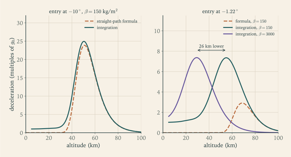
| \(-1.22^\circ\) | \(2.9\,g_0\) | \(7.4\,g_0\) | \(68.7\ \mathrm{km}\) | \(54.9\ \mathrm{km}\) | \(-6.1^\circ\) |
Steep entries. At \(-30^\circ\) and \(-10^\circ\) the formula is within \(3\) and \(4\) percent. The integration is slightly higher because gravity, which the formula dropped, speeds the body up a little on the way down.
Shallow entries. Below about \(5^\circ\) the formula fails, and it fails in the unsafe direction: at the upper stage’s \(-1.22^\circ\) it predicts \(2.9\,g_0\) where the integration gives \(7.4\,g_0\) . The last column shows why. A body entering shallowly at close to circular speed is nearly in orbit: the curvature term \(v^2/r\) supports most of its weight. As drag slows it, that support goes, gravity bends the path downward, and by the time the body reaches the denser air it is descending at \(6^\circ\) whatever angle it began with. Assumption (i), the straight path, is the one that broke. The peak deceleration stops falling as the entry is made shallower: it is \(7.8\,g_0\) at \(-2^\circ\) and stays between \(7.3\) and \(7.5\,g_0\) for every entry angle from \(-1.5^\circ\) to \(-0.7^\circ\) .
Does the similarity survive? Repeat the \(-1.22^\circ\) entry with \(\beta=3000\ \mathrm{kg/m^2}\) . The peak is \(7.37\,g_0\) against \(7.36\,g_0\) , and it occurs at \(29.3\ \mathrm{km}\) against \(54.9\ \mathrm{km}\) : lower by \(25.6\ \mathrm{km}\) , where Proposition 12.2 predicts \(H\ln20=25.5\ \mathrm{km}\) . The formula of Proposition 12.1 does not survive a shallow entry. The independence from \(\beta\) does.
Against experience. A summary of entry practice gives \(8\) to \(9\,g_0\) for a purely ballistic return from low orbit, reduced to \(4\) to \(5\,g_0\) when the capsule flies with a little lift (Wikipedia, “Atmospheric entry”; see sources). The model’s \(7.4\,g_0\) is somewhat below the ballistic range. Its scale height of \(8.5\ \mathrm{km}\) is an average for the lower atmosphere; the air at \(55\ \mathrm{km}\) thins out faster than that, and a shorter scale height gives a sharper pulse. Example 12.6 repeats the integration with tabulated standard densities and finds \(7.3\) to \(8.0\,g_0\) .
Figure 12.1 shows the deceleration against altitude for a steep and a shallow entry and for the two bodies.
12.5 Heat: how much reaches the body
The kinetic energy leaves the body as work done against drag, and that work is done on the air. A body moving at many times the speed of sound cannot push the air aside gently. A shock wave stands ahead of it, and the air passing through the shock is compressed and heated to thousands of kelvin within a layer a few centimetres to a few tens of centimetres thick. Most of that hot gas flows around the body and away, taking its energy with it. A small fraction of the energy is conducted from the hot layer into the surface. The heating of an entering body is caused by this compressed layer of gas. Friction on the skin is a minor contributor.
The stagnation point. The heating is greatest at the point on the nose where the flow is brought to rest. For a blunt axisymmetric nose of radius \(r_n\) a widely used correlation gives the heat flux there as a coefficient times \(\sqrt{p_s/r_n}\) times the difference in specific enthalpy between the stagnated gas and the gas at the wall, where \(p_s\) is the pressure at the stagnation point; for air the coefficient is \(0.1113\ \mathrm{kg/(s\cdot m^{3/2}\cdot atm^{1/2})}\) , fitted to boundary-layer computations over pressures from \(0.001\) to \(100\) atmospheres (Sutton and Graves report; see sources). Two substitutions turn it into a form that uses only the quantities of this chapter. At high speed the stagnation pressure is close to the momentum flux of the oncoming stream, \(p_s\approx\rho v^2\) . And by the steady-flow energy equation of Chapter 4, gas brought to rest from speed \(v\) gains the enthalpy \(v^2/2\) , beside which the enthalpy of gas at a cool wall is negligible. Then
in \(\mathrm{W/m^2}\) when \(\rho\) , \(r_n\) , and \(v\) are in SI units. The time integral of the flux, \(Q_w=\int\dot q_w\,\mathrm dt\) , is the heat load in \(\mathrm{J/m^2}\) .
What the scaling says. The flux goes as the cube of the speed, so heating is concentrated early, while the body is still fast. It goes as the square root of the density, so a body that decelerates high up, in thin air, is heated less. And it goes inversely as the square root of the nose radius.
Proposition 12.3 (heating on the straight path). Under the assumptions of Proposition 12.1, with \(\dot q_w\) proportional to \(\sqrt{\rho/r_n}\,v^3\) , the flux is greatest where \(\rho H=\tfrac13\beta\sin\lvert\theta_e\rvert\) , which is \(H\ln3=9.3\ \mathrm{km}\) above the altitude of peak deceleration, at the speed \(v_{\mathrm{entry}}\exp(-\tfrac16)\) . The peak flux is proportional to \(\sqrt{\beta\sin\lvert\theta_e\rvert/r_n}\) and the heat load to \(\sqrt{\beta/(r_n\sin\lvert\theta_e\rvert)}\) :
Proof. By Proposition 12.1, \(\sqrt\rho\,v^3\) equals \(v_{\mathrm{entry}}^3\sqrt\rho\exp\bigl(-3\rho H/(2\beta\sin\lvert\theta_e\rvert)\bigr)\) . Its logarithm, \(\tfrac12\ln\rho-3\rho H/(2\beta\sin\lvert\theta_e\rvert)\) , has zero derivative in \(\rho\) where \(\rho H=\tfrac13\beta\sin\lvert\theta_e\rvert\) ; there the exponent of the velocity formula is \(-\tfrac16\) , and the density is a third of its value at peak deceleration. For the heat load, \(\mathrm dt=-\mathrm dz/(v\sin\lvert\theta_e\rvert)\) and \(\mathrm dz=-H\,\mathrm d\rho/\rho\) , so \(Q_w\) is the constant times \((H v_{\mathrm{entry}}^2/(\sqrt{r_n}\sin\lvert\theta_e\rvert))\int_0^{\rho_{\mathrm{SL}}}\rho^{-1/2}\exp(-\rho H/(\beta\sin\lvert\theta_e\rvert))\,\mathrm d\rho\) . Extending the upper limit to infinity, which changes nothing when the peak is well above the ground, the integral is \(\sqrt{\pi\beta\sin\lvert\theta_e\rvert/H}\) .
The two proportionalities pull opposite ways in the entry angle. A steep entry gives a high flux for a short time and a small total. A shallow one gives a lower flux for much longer and a larger total. A designer who must keep a surface below some temperature wants a low flux; one who must absorb the heat in a limited mass of material wants a low load. No entry angle serves both.
Why bluntness helps. It helps three times over. A larger nose radius lowers the flux directly, as \(1/\sqrt{r_n}\) . A blunt shape has high drag, so a low ballistic coefficient, so it decelerates higher up in thinner air, and both the flux and the load fall as \(\sqrt\beta\) . And the reason behind both: a blunt nose holds its shock wave off at a distance, so the energy is deposited in a thick layer of gas of which only the innermost part touches the surface, while a slender pointed body keeps its shock close to the skin. The discovery that the heat load on an entering body is inversely proportional to its drag coefficient, so that a blunt, high-drag shape makes the best heat shield, was the result of the analysis cited in Section 12.2 (Wikipedia, “Atmospheric entry”; see sources).
Common mistake. Reasoning that a sharp, low-drag shape “slips through” and so heats less. It slips through the upper atmosphere without slowing, arrives fast in dense air, and takes its heating there, on a tip of small radius. Low drag is the wrong goal for a body that needs to get rid of energy.
Example 12.4: Flux, load, and nose radius
Inputs. The body of Example 12.2 with \(\beta=150\ \mathrm{kg/m^2}\) and a nose radius \(r_n=1.5\ \mathrm m\) (illustrative), entering at \(7894\ \mathrm{m/s}\) .
Peak flux at \(-10^\circ\) . By Proposition 12.3 the flux peaks at \(50.9+9.3=60.2\ \mathrm{km}\) , where \(\rho=(1.217)\exp(-60.2/8.5)=1.02\times10^{-3}\ \mathrm{kg/m^3}\) and \(v=7894\exp(-\tfrac16)=6682\ \mathrm{m/s}\) :
The integration of Example 12.3 gives \(1.40\ \mathrm{MW/m^2}\) at \(60.0\ \mathrm{km}\) .
Across entry angles.
| Entry angle | Peak flux, formula | Peak flux, integration | Heat load, formula | Heat load, integration |
|---|---|---|---|---|
| \(-30^\circ\) | \(2.31\ \mathrm{MW/m^2}\) | \(2.39\ \mathrm{MW/m^2}\) | \(25.2\ \mathrm{MJ/m^2}\) | \(25.4\ \mathrm{MJ/m^2}\) |
| \(-10^\circ\) | \(1.36\ \mathrm{MW/m^2}\) | \(1.40\ \mathrm{MW/m^2}\) | \(42.7\ \mathrm{MJ/m^2}\) | \(42.5\ \mathrm{MJ/m^2}\) |
| \(-5^\circ\) | \(0.96\ \mathrm{MW/m^2}\) | \(1.00\ \mathrm{MW/m^2}\) | \(60.3\ \mathrm{MJ/m^2}\) | \(58.7\ \mathrm{MJ/m^2}\) |
| \(-1.22^\circ\) | not valid | \(0.56\ \mathrm{MW/m^2}\) | not valid | \(102.6\ \mathrm{MJ/m^2}\) |
From the steepest entry to the shallowest the peak flux falls by a factor of four and the load rises by a factor of four.
Nose radius. Doubling the radius lowers the flux by \(\sqrt2=1.41\) at every instant. A nose of radius \(0.1\ \mathrm m\) in place of \(1.5\ \mathrm m\) raises it by \(\sqrt{15}=3.9\) .
The denser body. For \(\beta=3000\ \mathrm{kg/m^2}\) at \(-1.22^\circ\) the integration gives a peak flux of \(2.46\ \mathrm{MW/m^2}\) and a load of \(514\ \mathrm{MJ/m^2}\) , larger by factors of \(4.4\) and \(5.0\) , on either side of the \(\sqrt{20}=4.5\) that Proposition 12.3 gives for a steep entry. The two bodies of Example 12.3 felt the same deceleration. They do not feel the same heat.
12.6 Lift, and the corridor between two failures
A ballistic return from orbit costs seven to nine times standard gravity. People have flown it, but vehicles that carry them are built to do better, and they do it with a small amount of lift.
Equilibrium glide. Give the body a lift \(L\) , directed upward, and let it fly a path so shallow that \(\theta\approx0\) and \(\dot\theta\approx0\) . The second equation of Proposition 7.1, with no thrust, then says that the lift carries whatever part of the weight the curvature term does not:
The deceleration is the drag per unit mass, and drag is lift divided by the lift-to-drag ratio \(L/D\) , a property of the body’s shape and attitude. Hence
At circular speed the right side is zero. As the vehicle slows, lift takes over from curvature, and the deceleration rises smoothly toward \(g/(L/D)\) . Lift lets the vehicle stay high, in thin air, until it has slowed, instead of plunging into dense air while still fast.
Example 12.5: Deceleration on a lifting glide
Inputs. The Apollo command module flew with an average \(L/D=0.368\) (Wikipedia, “Atmospheric entry”; see sources). Take \(r=R_E+60\ \mathrm{km}\) , where \(g=9.616\ \mathrm{m/s^2}\) and the circular speed is \(7868\ \mathrm{m/s}\) .
| Speed as a fraction of circular speed | \(0.9\) | \(0.7\) | \(0.5\) | \(0.25\) | toward \(0\) |
|---|---|---|---|---|---|
| Deceleration | \(0.51\,g_0\) | \(1.36\,g_0\) | \(2.00\,g_0\) | \(2.50\,g_0\) | \(2.66\,g_0\) |
Reading the table. With lift equal to about a third of drag, the peak deceleration of an idealized glide is \(2.7\,g_0\) instead of \(7.4\,g_0\) . Real capsule entries, which do not hold all of their lift upward and do not fly so shallow a path, are reported at \(4\) to \(5\,g_0\) , between the two.
The corridor. An entry can fail on either side. Too steep, and the deceleration rises with the sine of the angle (Proposition 12.1) and the heat flux with its square root (Proposition 12.3): the integration of Example 12.3 passes \(10\,g_0\) , the limit the same article quotes for crews returning to Earth, at an entry angle of \(-3.4^\circ\) . Too shallow, and the heat load grows, the point of landing becomes sensitive to every uncertainty in the drag, and a vehicle arriving faster than circular speed can leave the atmosphere again before it has slowed enough to be captured. The band of entry angles between the two failures is the entry corridor. Lift widens it, by giving the vehicle a means of correcting its path after entry has begun. Flying within it is a guidance problem of the kind met in Chapter 10, with the direction of the lift as the control, and it is outside this course.
12.7 The upper stage comes down
The stage has no heat shield, no lift, and no control. The purpose of the disposal burn is to make sure that it comes down promptly, in a known region, and in pieces small enough not to matter.
Example 12.6: Disposal of the reference launcher’s upper stage
The object. After the disposal burn the stage is empty: \(1984\ \mathrm{kg}\) , a cylinder \(3\ \mathrm m\) across and about \(6\ \mathrm m\) long, tumbling. Its drag area is uncertain. End-on, with \(C_DS\) of about \(7\ \mathrm{m^2}\) , its ballistic coefficient is \(280\ \mathrm{kg/m^2}\) ; broadside, with about \(20\ \mathrm{m^2}\) , it is \(100\ \mathrm{kg/m^2}\) (illustrative bounds). Take \(r_n=1.5\ \mathrm m\) , the radius of the body.
Timeline. The burn of \(102.3\ \mathrm{m/s}\) is made at \(400\ \mathrm{km}\) . Kepler’s equation (Section 8.9) gives \(31.7\ \mathrm{min}\) from the burn to the entry interface, during which the stage travels \(126^\circ\) around the Earth. It crosses \(120\ \mathrm{km}\) at \(7894\ \mathrm{m/s}\) and \(-1.22^\circ\) .
The entry, from the integration of Example 12.3:
| Quantity | \(\beta=100\ \mathrm{kg/m^2}\) | \(\beta=280\ \mathrm{kg/m^2}\) |
|---|---|---|
| Peak deceleration | \(7.35\,g_0\) | \(7.36\,g_0\) |
| Time of the peak after the interface | \(306\ \mathrm s\) | \(367\ \mathrm s\) |
| Altitude and speed at the peak | \(58.4\ \mathrm{km}\) , \(3.38\ \mathrm{km/s}\) | \(49.6\ \mathrm{km}\) , \(3.37\ \mathrm{km/s}\) |
| Peak heat flux at the stagnation point | \(461\ \mathrm{kW/m^2}\) at \(75.5\ \mathrm{km}\) | \(767\ \mathrm{kW/m^2}\) at \(66.6\ \mathrm{km}\) |
| Heat load at the stagnation point | \(82\ \mathrm{MJ/m^2}\) | \(144\ \mathrm{MJ/m^2}\) |
| Time above \(1\,g_0\) | \(362\ \mathrm s\) | \(269\ \mathrm s\) |
| Reaches \(10\ \mathrm{km}\) altitude | \(554\ \mathrm s\) and \(2256\ \mathrm{km}\) from the interface | \(523\ \mathrm s\) and \(2735\ \mathrm{km}\) |
The two columns differ in altitude by \(8.8\ \mathrm{km}\) at the peak, and \(H\ln2.8=8.75\ \mathrm{km}\) .
What the heat does. The second stage’s tank walls in Example 6.9 are aluminium alloy at the minimum gauge of \(2\ \mathrm{mm}\) (illustrative), of density \(2840\ \mathrm{kg/m^3}\) : \(5.68\ \mathrm{kg}\) of metal behind each square metre of skin. By Example 12.1, bringing that to its melting point and melting it takes \((5.68)(0.965)=5.5\ \mathrm{MJ/m^2}\) . The heat load at the stagnation point is \(15\) to \(26\) times that. Elsewhere on the body the load is lower by a factor of several, and still well above what the wall can absorb. Nor can the wall shed the heat by radiating it: a surface radiating at the rate \(\sigma_{\mathrm{SB}}T_{\mathrm{wall}}^4\) , with the Stefan-Boltzmann constant \(\sigma_{\mathrm{SB}}=5.670\times10^{-8}\ \mathrm{W/(m^2\cdot K^4)}\) (NIST; see sources), balances \(461\ \mathrm{kW/m^2}\) only at \(T_{\mathrm{wall}}=(461\,000/5.670\times10^{-8})^{1/4}=1689\ \mathrm K\) , far above the melting point. In the integration the wall at the stagnation point has received its \(5.5\ \mathrm{MJ/m^2}\) when only \(4\) to \(7\) percent of the heat load has arrived and the deceleration is still under a tenth of \(g_0\) . The exponential atmosphere puts that moment a minute after the interface; the tabulated atmosphere used below puts it at \(160\ \mathrm s\) , near \(95\ \mathrm{km}\) . The thin structure melts early in the heat pulse, long before the peak of deceleration, and the stage comes apart. Compact, dense parts such as the engine have much larger ballistic coefficients and thermal mass, and some of them may reach the surface; this model cannot say which.
Where. Between the two ballistic coefficients the point of descent moves by \(479\ \mathrm{km}\) along the track, and fragments, each with its own \(\beta\) , will be spread over more than that. This is the reason for the choice made in Chapter 9. A perigee of \(50\ \mathrm{km}\) gives an entry angle of \(-1.22^\circ\) . A perigee of \(100\ \mathrm{km}\) would save \(15\ \mathrm{m/s}\) of burn, but the angle would be \(-0.65^\circ\) and the same two bodies would come down \(1200\ \mathrm{km}\) apart; a perigee at the surface, costing \(15\ \mathrm{m/s}\) more, steepens the entry to \(-1.60^\circ\) and narrows the spread to \(340\ \mathrm{km}\) . A disposal burn buys a predictable place of descent, and that is why it is timed to end over an empty ocean.
Energy accounts. Of the stage’s \(62\ \mathrm{GJ}\) , melting all \(1984\ \mathrm{kg}\) of it would take \(1.9\ \mathrm{GJ}\) , three percent. The other \(97\) percent, at least, goes into the air.
How far to trust the altitudes and times. The exponential atmosphere was shown in Section 7.4 to be twice too dense at \(30\ \mathrm{km}\) , and the error grows with height: against a table of the standard atmosphere (PDAS standard atmosphere table; see sources) it is too dense by a factor of \(3.4\) at \(60\ \mathrm{km}\) , \(5\) at \(80\ \mathrm{km}\) , \(17\) at \(100\ \mathrm{km}\) , and \(40\) at \(120\ \mathrm{km}\) . Proposition 12.2 says what a constant factor would do. It is equivalent to a ballistic coefficient too small by that factor: the histories of speed, deceleration, and heat flux are unchanged, and every event is placed too high, by \(H\) times the logarithm of the factor, about \(6\ \mathrm{km}\) for a factor of two and \(12\ \mathrm{km}\) for a factor of four. The factor is not constant, so the integration was repeated with the tabulated densities, interpolated in their logarithm:
| Quantity, tabulated atmosphere | \(\beta=100\ \mathrm{kg/m^2}\) | \(\beta=280\ \mathrm{kg/m^2}\) |
|---|---|---|
| Peak deceleration | \(7.3\,g_0\) at \(418\ \mathrm s\) and \(47.3\ \mathrm{km}\) | \(8.0\,g_0\) at \(481\ \mathrm s\) and \(38.7\ \mathrm{km}\) |
| Peak heat flux | \(474\ \mathrm{kW/m^2}\) at \(65.0\ \mathrm{km}\) | \(760\ \mathrm{kW/m^2}\) at \(57.2\ \mathrm{km}\) |
| Heat load | \(82\ \mathrm{MJ/m^2}\) | \(144\ \mathrm{MJ/m^2}\) |
| Wall capacity reached | \(160\ \mathrm s\) , at \(95\ \mathrm{km}\) | \(160\ \mathrm s\) , at \(95\ \mathrm{km}\) |
The peak comes about \(110\ \mathrm s\) later and \(11\ \mathrm{km}\) lower than in the exponential model, and the stage flies some \(850\ \mathrm{km}\) farther before it is down. The heat fluxes and loads hardly move, and the conclusion about the wall does not move at all. The peak deceleration is no longer the same for the two bodies, because Proposition 12.2 needs an exponential atmosphere: it is the error in the scale height, noted in Example 12.3, that changes the peak itself.
12.8 The design loop, run to convergence
The entry closes the list of things the vehicle does. What remains is to assemble the vehicle itself. Its numbers at present are scattered: Revision A in Chapter 2, its engines and tanks in Chapters 3 to 6, its flight in Chapter 7, a resized Revision B in Chapter 9 that Chapters 3 to 6 never saw, a better steering law in Chapter 10 that neither revision used, a fairing that Section 6.8 costed and no revision carries.
The loop. Every step has been done once already, in some chapter:
- Requirements (fixed since Chapter 1): \(5000\ \mathrm{kg}\) to a circular orbit at \(400\ \mathrm{km}\) , inclination \(28.5^\circ\) , two stages burning kerosene and oxygen.
- Velocity budget (Definition 9.2): what the stages must supply with the payload on board.
- Staging (Theorem 2.4): the split of that velocity between the stages that minimizes liftoff mass.
- Propulsion (Chapters 3 to 5): thrusts from the thrust-to-weight ratios, flows from the specific impulses, throats and exits from the chamber conditions.
- Structure (Chapter 6): tank volumes, engine masses, and the estimate that tests the structural coefficients.
- Ascent (Chapters 7 and 10): the model flight, with the gravity turn and the tangent law.
- Orbit (Chapters 8 and 9): the transfer, the disposal burn.
- Control (Chapter 11): the vehicle’s stability and gimbal demand at maximum dynamic pressure.
- Entry (this chapter): the stage’s return.
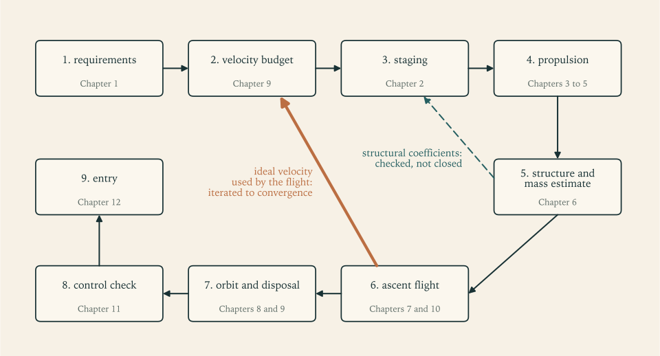
Step 6 feeds step 2: the losses in the budget come from the flight, and the flight depends on the vehicle that the budget sized. So the loop is run until its numbers stop changing. Figure 12.2 shows it.
What the final pass uses that Revision B did not. Four things.
The budget is taken from the vehicle’s own flight. Chapter 9 built its budget from Revision A’s losses on a non-rotating Earth and a rotation credit, and found that convention cautious by about \(25\ \mathrm{m/s}\) . Here the budget is the ideal velocity that the vehicle’s own model flight uses to reach the parking orbit, on the rotating ground of Example 9.8, plus the transfer, the allowance, and the reserve. At convergence the model flight ends with exactly its provision in hand.
The flight uses Chapter 10’s steering: the tangent law on the second stage and the best pitch-over angle.
The fairing is carried. Its \(570\ \mathrm{kg}\) (Section 6.8, illustrative) rides on the first stage and is dropped at staging, so it is counted as first-stage inert mass. Because it is a fixed mass and not a fraction, the first stage’s effective coefficient depends on the stage’s size and is found by iteration within each pass.
The allowance is recomputed for the flight flown. Chapter 9’s allowance has two large items, and each is a gap: the median loss of the six cited vehicles less the loss in the model flight. Chapter 9 took the model losses from Revision A’s constant-angle ascent and found \(116.0-3.5=112.5\ \mathrm{m/s}\) for steering and \(122.5-49.0=73.5\ \mathrm{m/s}\) for drag. Revision C’s flight is a different flight. Steered by the tangent law, it has a steering loss of \(12.9\ \mathrm{m/s}\) ; flying a flatter path, and lighter on the same cross-section, it has a drag loss of \(58.2\ \mathrm{m/s}\) . Both are the integrals of Proposition 7.2 taken against the velocity relative to the ground, which is the velocity the air sees. The same rule therefore gives
Carrying Chapter 9’s two figures forward unchanged would provide for the medians and \(19\ \mathrm{m/s}\) besides, and the allowance could no longer be described as calibrated to them. The pitch-over item is the impulse of the flight flown. The loop therefore recomputes the allowance at every pass, from the flight just made.
What is kept. The specific impulses, \(285\) , \(315\) , and \(345\ \mathrm s\) . The structural coefficients of the stage hardware, \(0.06\) and \(0.08\) , with the disposal reserve in the second as in Section 9.8. The thrust-to-weight ratios \(1.30\) and \(0.90\) . The reserve of \(100\ \mathrm{m/s}\) . The two medians and the rule that turns them into an allowance. And the allowance’s throttle item, \(3.1\ \mathrm{m/s}\) , which is Chapter 7’s figure for Revision A and was not flown again.
Example 12.7: Revision C
Starting point. Revision B, flown with the tangent law in Example 10.10: ideal velocity used \(8858.7\ \mathrm{m/s}\) , with a steering loss of \(11.5\ \mathrm{m/s}\) and a drag loss of \(59.1\ \mathrm{m/s}\) , so that the rule gives an allowance of \(104.5+63.4+3.1+3.1=174.1\ \mathrm{m/s}\) .
The passes.
| Pass | Budget | Liftoff mass | Ideal velocity used by the new vehicle | Left after the transfer | Allowance and reserve for the new flight |
|---|---|---|---|---|---|
| \(1\) | \(9248.5\ \mathrm{m/s}\) | \(161\,915\ \mathrm{kg}\) | \(8871.7\ \mathrm{m/s}\) | \(258.8\ \mathrm{m/s}\) | \(273.2\ \mathrm{m/s}\) |
| \(2\) | \(9260.6\ \mathrm{m/s}\) | \(162\,957\ \mathrm{kg}\) | \(8870.5\ \mathrm{m/s}\) | \(274.6\ \mathrm{m/s}\) | \(273.6\ \mathrm{m/s}\) |
| \(3\) | \(9259.8\ \mathrm{m/s}\) | \(162\,884\ \mathrm{kg}\) | \(8870.5\ \mathrm{m/s}\) | \(273.5\ \mathrm{m/s}\) | \(273.6\ \mathrm{m/s}\) |
| \(4\) | \(9259.8\ \mathrm{m/s}\) | \(162\,889\ \mathrm{kg}\) | \(8870.5\ \mathrm{m/s}\) | \(273.6\ \mathrm{m/s}\) | \(273.6\ \mathrm{m/s}\) |
| \(5\) | \(9259.8\ \mathrm{m/s}\) | \(162\,889\ \mathrm{kg}\) | \(8870.5\ \mathrm{m/s}\) | \(273.6\ \mathrm{m/s}\) | \(273.6\ \mathrm{m/s}\) |
The first budget is \(8858.7+115.7+174.1+100.0=9248.5\ \mathrm{m/s}\) . The vehicle sized for it carries the fairing, flies a slightly different path, and uses \(13\ \mathrm{m/s}\) more than Revision B did, so its flight ends \(14\ \mathrm{m/s}\) short of the allowance and reserve that its own losses call for. The second pass corrects that and overshoots by one; the changes then fall by a factor of more than ten per pass, and between the fourth and fifth passes the liftoff mass moves by less than a kilogram. The loop has converged: the flight ends with exactly its own allowance and reserve in hand. The fifth pass is Revision C.
The budget of Revision C.
| Line | Value | Kind |
|---|---|---|
| Ideal velocity used by the model flight to the \(200\ \mathrm{km}\) parking orbit | \(8870.5\ \mathrm{m/s}\) | model output |
| Transfer to \(400\ \mathrm{km}\) | \(115.7\ \mathrm{m/s}\) | two-body result |
| Allowance: steering gap, \(116.0-12.9\) | \(103.1\ \mathrm{m/s}\) | calibrated to cited data |
| Allowance: drag gap, \(122.5-58.2\) | \(64.3\ \mathrm{m/s}\) | calibrated to cited data |
| Allowance: pitch-over impulse | \(3.1\ \mathrm{m/s}\) | model output |
| Allowance: throttle to \(5\,g_0\) | \(3.1\ \mathrm{m/s}\) | model output (Chapter 7) |
| Reserve | \(100.0\ \mathrm{m/s}\) | design choice |
| Total \(\Delta v_{\mathrm{req}}\) | \(9259.8\ \mathrm{m/s}\) |
The three revisions.
| Quantity | Revision A (Chapter 2) | Revision B (Chapter 9) | Revision C |
|---|---|---|---|
| Velocity budget | \(9400\ \mathrm{m/s}\) , provisional | \(9306.3\ \mathrm{m/s}\) | \(9259.8\ \mathrm{m/s}\) |
| Stage 1 exhaust velocity in the staging | \(2942.0\ \mathrm{m/s}\) | \(3028.4\ \mathrm{m/s}\) | \(3027.1\ \mathrm{m/s}\) |
| Stage 1 coefficient in the staging | \(0.06\) | \(0.06\) | \(0.06403\) , with the fairing |
| Stage 2 coefficient in the staging | \(0.08\) | \(0.08246\) | \(0.08246\) |
| Mass ratios | \(4.359\) , \(4.473\) | \(4.412\) , \(4.146\) | \(4.251\) , \(4.230\) |
| Liftoff mass | \(177\,812\ \mathrm{kg}\) | \(162\,985\ \mathrm{kg}\) | \(162\,889\ \mathrm{kg}\) |
| Stage 2 stack at ignition | \(32\,045\ \mathrm{kg}\) | \(28\,898\ \mathrm{kg}\) | \(29\,799\ \mathrm{kg}\) |
| Stage 1 propellant | \(137\,021\ \mathrm{kg}\) | \(126\,041\ \mathrm{kg}\) | \(124\,569\ \mathrm{kg}\) |
| Stage 1 hardware; fairing | \(8746\ \mathrm{kg}\) ; none | \(8045\ \mathrm{kg}\) ; none | \(7951\ \mathrm{kg}\) ; \(570\ \mathrm{kg}\) |
| Stage 2 propellant | \(24\,881\ \mathrm{kg}\) | \(21\,927\ \mathrm{kg}\) | \(22\,754\ \mathrm{kg}\) |
| Stage 2 hardware; disposal reserve | \(2164\ \mathrm{kg}\) ; none | \(1912\ \mathrm{kg}\) ; \(59\ \mathrm{kg}\) | \(1984\ \mathrm{kg}\) ; \(61\ \mathrm{kg}\) |
| Payload fraction | \(2.81\) percent | \(3.07\) percent | \(3.07\) percent |
Reconciling B and C. The two differ by less than a tenth of a percent in liftoff mass, and that near-equality hides two changes of two percent each with opposite signs. The budget fell by \(46.4\ \mathrm{m/s}\) , from the rotation convention, the better steering, and the allowance recomputed for it, and by the multiplier of Chapter 2 that is worth \(1-\exp[-(4.49\times10^{-4})(46.4)]=2.1\) percent of liftoff mass: Revision B resized for the new budget alone would weigh \(159\,626\ \mathrm{kg}\) . The slightly lower flight-average exhaust velocity of the new first stage adds \(0.1\) percent. The fairing, \(570\ \mathrm{kg}\) of first-stage inert mass, takes back \(2.0\) percent. The fairing also changed the shape of the optimum: with a heavier first stage, Theorem 2.4 moves velocity onto the second, whose mass ratio rises from \(4.146\) to \(4.230\) and whose stack grows by \(0.9\ \mathrm t\) while the first stage’s propellant load falls by \(1.5\ \mathrm t\) .
Does the mass estimate still support the coefficients? Applying the rules of Example 6.9 to Revision C’s loads gives \(6949\ \mathrm{kg}\) for the first stage’s hardware, or \(8090\ \mathrm{kg}\) with \(20\) percent growth, against the \(7951\ \mathrm{kg}\) carried: coefficients of \(0.053\) and \(0.061\) against \(0.06\) . For the second stage, \(1575\ \mathrm{kg}\) or \(1822\ \mathrm{kg}\) with growth against \(1984\ \mathrm{kg}\) : \(0.065\) and \(0.074\) against \(0.08\) . The position is the one Chapter 6 reported: the estimate is consistent with the assumed coefficients and does not derive them, since it reaches them only through an illustrative factor on tank mass and an illustrative growth allowance. This return arrow of the loop is checked, not closed.
12.9 Every number, and what it rests on
The tables below are the design review’s record of Revision C. Each row names the chapter that produced the number and the assumption it would fall with. The last column sorts the numbers into kinds: requirement; choice, a decision that could have been made otherwise; illustrative input, a value assumed without derivation; derived, a consequence of the rows above it by a theorem or formula of the course; model output, the result of a numerical model whose limits were stated where it was built; and calibrated, taken from cited data on real vehicles.
Mass.
| Quantity | Value | Derived in | Rests on | Kind |
|---|---|---|---|---|
| Payload | \(5000\ \mathrm{kg}\) | Chapter 1 | the mission | requirement |
| Velocity budget | \(9259.8\ \mathrm{m/s}\) | Example 12.7, by Definition 9.2 | the model flight, the allowance, the reserve | model output plus calibrated plus choice |
| Stage 1 flight-average exhaust velocity | \(3027.1\ \mathrm{m/s}\) (\(308.7\ \mathrm s\) ) | Section 7.6; flown in Example 12.7 | \(285\) and \(315\ \mathrm s\) | model output from illustrative inputs |
| Stage 2 exhaust velocity | \(3383.3\ \mathrm{m/s}\) (\(345\ \mathrm s\) ) | Example 5.8 | the model gas at area ratio \(140\) , delivered at \(97.5\) percent of the model’s ideal | illustrative input |
| Stage 1 hardware coefficient | \(0.06\) | assumed in Chapter 2; tested in Example 6.9 | tank factor of \(2\) and growth of \(20\) percent | illustrative input |
| Stage 2 hardware coefficient | \(0.08\) | assumed in Chapter 2; tested in Example 6.9 | the same; the one real stage of this size is at \(0.085\) | illustrative input |
| Disposal reserve | \(61\ \mathrm{kg}\) | Section 9.8 | impulsive burn of \(102.3\ \mathrm{m/s}\) by the empty stage | derived |
| Fairing | \(570\ \mathrm{kg}\) | Section 6.8 | \(10\ \mathrm{kg/m^2}\) of shell; dropped at staging | illustrative input |
| Mass ratios | \(4.251\) and \(4.230\) | Theorem 2.4 | the rows above | derived |
| Stage velocity increments | \(4380.5\) and \(4879.3\ \mathrm{m/s}\) | Proposition 1.2 | the rows above | derived |
| Liftoff mass | \(162\,889\ \mathrm{kg}\) | Example 12.7 | everything above | derived |
| Payload fraction | \(3.07\) percent | Definition 2.1 | everything above | derived |
Propulsion.
| Quantity | Stage 1 | Stage 2 | Derived in | Rests on | Kind |
|---|---|---|---|---|---|
| Thrust-to-weight ratio at ignition | \(1.30\) | \(0.90\) | Chapter 2; tested in Example 7.7 and Section 7.10 | the trade of gravity loss against engine mass and loads | choice |
| Thrust | \(2077\ \mathrm{kN}\) at sea level, \(2295\ \mathrm{kN}\) in vacuum | \(263.0\ \mathrm{kN}\) | Definition 1.5; Section 7.5 | the ratio above; \(285\) , \(315\) , \(345\ \mathrm s\) | derived |
| Mass flow | \(743.0\ \mathrm{kg/s}\) | \(77.74\ \mathrm{kg/s}\) | Definition 1.3 | the specific impulses | derived |
| Burn time | \(167.7\ \mathrm s\) | \(292.7\ \mathrm s\) available | Section 1.6 | constant flow | derived |
| Engines | three of \(692.2\ \mathrm{kN}\) at sea level | one | Section 3.9 | no engine-out capability | choice |
| Chamber | \(10\ \mathrm{MPa}\) , \(3600\ \mathrm K\) , \(c^\ast=1759\ \mathrm{m/s}\) | the same | Chapters 4 and 5 | single-\(\gamma\) model gas of molar mass \(23\ \mathrm{g/mol}\) | illustrative input |
| Throat area | \(0.1307\ \mathrm{m^2}\) in all | \(0.01367\ \mathrm{m^2}\) | Theorem 5.3 | choked flow; the model gas | derived |
| Area ratio | \(16.5\) | \(140\) | Example 5.8 | separation limit on the pad; size in vacuum | choice |
| Exit area | \(2.156\ \mathrm{m^2}\) in all | \(1.914\ \mathrm{m^2}\) | Example 5.8 | the two rows above | derived |
| Tank volume and column at \(3.0\ \mathrm m\) diameter | \(122.7\ \mathrm{m^3}\) , \(17.36\ \mathrm m\) | \(22.47\ \mathrm{m^3}\) , \(3.18\ \mathrm m\) , disposal propellant included | Example 6.1 | mixture ratio \(2.3\) ; bulk density \(1015\ \mathrm{kg/m^3}\) | derived from illustrative inputs |
| Pump power | \(15.7\ \mathrm{MW}\) | \(1.64\ \mathrm{MW}\) | Example 6.5 | pressure rise \(15\ \mathrm{MPa}\) ; efficiency \(0.7\) | derived from illustrative inputs |
| Engine mass | \(2118\ \mathrm{kg}\) | \(361\ \mathrm{kg}\) | Example 6.9 | engine thrust-to-weight of \(100\) (illustrative) and \(74.4\) (cited) | derived |
| Hardware mass: estimate, with growth, carried | \(6949\) , \(8090\) , \(7951\ \mathrm{kg}\) | \(1575\) , \(1822\) , \(1984\ \mathrm{kg}\) | Example 6.9 | see the mass table | model output against illustrative input |
Ascent, from the model flight of Revision C on the rotating ground.
| Quantity | Value | Derived in | Rests on | Kind |
|---|---|---|---|---|
| Pitch-over | \(2.45^\circ\) at \(20\ \mathrm s\) | Sections 7.7 and 10.8 | instantaneous rotation; its \(3.1\ \mathrm{m/s}\) is in the allowance | model output |
| Stage 1 steering | gravity turn, zero angle of attack | Sections 7.7 and 10.9 | structure spared at a cost of about \(13\ \mathrm{m/s}\) per degree forgone | choice |
| Maximum dynamic pressure | \(33.9\ \mathrm{kPa}\) at \(79.5\ \mathrm s\) , \(14.7\ \mathrm{km}\) , airspeed \(561\ \mathrm{m/s}\) | Section 7.4 | exponential atmosphere; no wind | model output |
| Staging | \(167.7\ \mathrm s\) , \(73.3\ \mathrm{km}\) , inertial speed \(3587\ \mathrm{m/s}\) | Section 7.8 | instantaneous, no coast | model output |
| Stage 2 steering | tangent law, pitch from \(23.9^\circ\) to \(-5.6^\circ\) at \(1.920\times10^{-3}\ \mathrm{s^{-1}}\) | Proposition 10.3; Example 10.7 | flat-Earth law on a round Earth, within \(0.07\ \mathrm{m/s}\) of the free optimum | model output |
| Cutoff in the parking orbit | \(449.3\ \mathrm s\) ; \(859\ \mathrm{kg}\) unburned | Section 7.9 | point mass; perfect steering | model output |
| Ideal velocity used | \(8870.5\ \mathrm{m/s}\) | Proposition 7.2 | all of the above | model output |
| Model loss lines of this flight | drag \(58.2\ \mathrm{m/s}\) , steering \(12.9\ \mathrm{m/s}\) , against ground-relative velocity | Proposition 7.2; Section 12.8 | constant drag coefficient \(0.3\) on \(7.07\ \mathrm{m^2}\) ; stage 1 at zero angle of attack | model output |
| Allowance | \(173.6\ \mathrm{m/s}\) | Section 9.9; Section 12.8 | medians of six cited vehicles, less the two lines above | calibrated |
| Reserve | \(100.0\ \mathrm{m/s}\) | Section 9.9 | judgment | choice |
| Sensed acceleration | \(6.11\,g_0\) at stage 1 burnout unthrottled; \(3.39\,g_0\) at cutoff | Section 1.6; Section 7.10 | throttle to \(5\,g_0\) provided for | derived |
Orbit.
| Quantity | Value | Derived in | Rests on | Kind |
|---|---|---|---|---|
| Parking orbit | circular, \(200\ \mathrm{km}\) , \(7784.3\ \mathrm{m/s}\) | Definition 7.1; Section 9.7 | two-body motion; decay threshold of \(150\ \mathrm{km}\) | derived; choice of altitude |
| Rotation of the launch site | \(408.7\ \mathrm{m/s}\) eastward | Section 9.6 | latitude \(28.5^\circ\) , launch due east; in the flight, not a credit line | derived |
| Transfer | \(58.07+57.63=115.7\ \mathrm{m/s}\) in \(45.26\ \mathrm{min}\) | Proposition 9.1 | impulsive burns | derived |
| Target orbit | circular, \(400\ \mathrm{km}\) , \(7668.6\ \mathrm{m/s}\) , period \(92.56\ \mathrm{min}\) | Chapter 8 | two-body motion | requirement and derived |
| Disposal | \(102.3\ \mathrm{m/s}\) at \(400\ \mathrm{km}\) to a \(50\ \mathrm{km}\) perigee | Section 9.8 | empty stage; impulsive | derived |
Control and entry.
| Quantity | Value | Derived in | Rests on | Kind |
|---|---|---|---|---|
| Length | \(34.5\ \mathrm m\) | Example 11.1’s layout rules | illustrative arrangement | derived from illustrative inputs |
| Centre of mass and pitch inertia at maximum dynamic pressure | \(19.74\ \mathrm m\) from the nose; \(8.46\times10^{6}\ \mathrm{kg\cdot m^2}\) | Section 11.1 | rigid body, slender segments | model output |
| Aerodynamic moment \(M_\alpha\) | \(7.54\times10^{6}\ \mathrm{N\cdot m/rad}\) ; divergence doubles in \(0.73\ \mathrm s\) | Proposition 11.1; Definition 11.1 | slender-body theory, conical fairing | model output |
| Control moment \(M_\delta\) ; trim ratio | \(3.00\times10^{7}\ \mathrm{N\cdot m/rad}\) ; \(0.251\) | Section 11.3 | gimbal \(1\ \mathrm m\) below the tanks | model output |
| Gains for \(2.5\ \mathrm{rad/s}\) and damping ratio \(0.7\) | \(K_p=2.01\) , \(K_d=0.99\ \mathrm s\) | Section 11.4 | rigid body; ideal actuator | derived |
| Upper-stage entry | \(7894\ \mathrm{m/s}\) at \(-1.22^\circ\) , \(31.7\ \mathrm{min}\) after the burn | Chapter 8; Example 12.6 | two-body motion to \(120\ \mathrm{km}\) | derived |
| Peak deceleration of the stage | \(7.4\,g_0\) ; \(7.3\) to \(8.0\,g_0\) with tabulated densities | Example 12.6 | the atmosphere model; constant \(\beta\) | model output |
| Stagnation heat load | \(82\) to \(144\ \mathrm{MJ/m^2}\) against a wall capacity of \(5.5\ \mathrm{MJ/m^2}\) | Example 12.6 | cited heating correlation; \(\beta\) of \(100\) to \(280\ \mathrm{kg/m^2}\) | model output from illustrative inputs |
The control numbers are for Revision C at its own maximum dynamic pressure and are close to Chapter 11’s for Revision A: the vehicle is \(2.0\ \mathrm m\) shorter and \(9\) percent lighter at that instant, its divergence a little faster, its trim ratio a little higher. The wind simulation of Example 11.7 was not repeated.
Reading down the last columns is the point of the exercise. The derived rows are as good as the rows they depend on. The choices can be defended or changed. The weight of the design rests on a short list of illustrative inputs, three specific impulses and two structural coefficients, and on one calibration, the allowance.
12.10 What moves the answer, and what breaks first
A sized vehicle is a point estimate. The review’s last question is how far the point could be from the truth, and which error would be found first.
The measure. Freeze Revision C as built: its propellant loads, its engines, its hardware. Ask how much payload that vehicle can carry through the budget if one input turns out to differ from its assumed value. The answer comes from the rocket equation applied to both stages, as in Section 2.6, with the payload as the unknown. A structural coefficient is the hardware’s share of the stage, \(m_s/(m_s+m_p)\) , so with the propellant fixed a coefficient raised from \(\varepsilon\) to \(\varepsilon'\) means hardware of \(\varepsilon'm_p/(1-\varepsilon')\) .
Example 12.8: The payload at risk from each input
| Input | Plausible error | Source of the error bar | Change in payload |
|---|---|---|---|
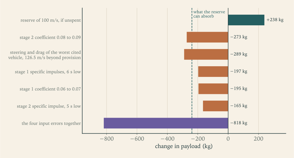
| Reserve, if entirely spent | \(100\ \mathrm{m/s}\) | Section 9.9 | \(+238\ \mathrm{kg}\) of capability in hand |
| Stage 2 hardware coefficient | \(0.08\) to \(0.09\) , that is \(+273\ \mathrm{kg}\) | Section 6.8 | \(-273\ \mathrm{kg}\) |
| Stage 2 hardware coefficient | to \(0.085\) , the cited real stage, that is \(+136\ \mathrm{kg}\) | Example 6.9 | \(-136\ \mathrm{kg}\) |
| Steering and drag beyond allowance and reserve | \(126.5\ \mathrm{m/s}\) , the worst of six cited vehicles | Section 9.9 | \(-289\ \mathrm{kg}\) |
| Stage 1 specific impulses | \(-6\ \mathrm s\) | Section 6.8 | \(-197\ \mathrm{kg}\) |
| Stage 1 hardware coefficient | \(0.06\) to \(0.07\) , that is \(+1425\ \mathrm{kg}\) | Section 6.8 | \(-195\ \mathrm{kg}\) |
| Stage 2 specific impulse | \(-5\ \mathrm s\) | Section 6.8 | \(-165\ \mathrm{kg}\) |
| Fairing | \(570\ \mathrm{kg}\) , if it weighed nothing | Section 6.8 | \(+82\ \mathrm{kg}\) |
| The four input errors together | \(-818\ \mathrm{kg}\) |
The exchange ratios behind the table. A kilogram of second-stage hardware costs a kilogram of payload. A kilogram of first-stage hardware costs \(0.14\ \mathrm{kg}\) . A metre per second of budget costs \(2.3\ \mathrm{kg}\) . A second of specific impulse on either stage is worth \(33\ \mathrm{kg}\) . These are Revision A’s ratios of Example 2.6 (\(1\) , \(0.13\) , \(2.4\) , and \(34\) to \(35\) ) almost unchanged, which is itself a finding: the design has moved by eight percent in mass since Chapter 2 and its sensitivities by less.
How the steering line is computed. Revision C’s model flight carries \(12.9+58.2=71.1\ \mathrm{m/s}\) of steering and drag loss; the allowance adds \(103.1+64.3=167.4\ \mathrm{m/s}\) ; so \(238.5\ \mathrm{m/s}\) is provided, which is the sum of the two medians by construction, or \(338.5\ \mathrm{m/s}\) with the reserve. The six cited vehicles lost \(169\) , \(173\) , \(221\) , \(277\) , \(283\) , and \(465\ \mathrm{m/s}\) . The provision covers three of them outright and five with the reserve. The sixth is \(126.5\ \mathrm{m/s}\) beyond it. The stage 2 coefficient rows count the disposal propellant with the stage’s propellant, as Section 9.8 did, and leave the disposal reserve as loaded.
Reading the table. The reserve is worth \(238\ \mathrm{kg}\) of payload. Three of the four input errors, taken singly, fall inside it, at \(165\) to \(197\ \mathrm{kg}\) . The fourth, the second stage’s coefficient, does not, at \(273\ \mathrm{kg}\) , and neither does an ascent like the worst of the cited vehicles. No two of them together are covered. All four together cost \(818\ \mathrm{kg}\) , three and a half times the reserve and a sixth of the payload. Combined as independent errors, by the root of the sum of their squares, they come to \(423\ \mathrm{kg}\) . Either way the honest statement of the design’s capability is not “\(5000\ \mathrm{kg}\) ” but “\(5000\ \mathrm{kg}\) if the inputs hold, and somewhere between \(4200\) and \(5200\ \mathrm{kg}\) if they do not”. Figure 12.3 sets the bars side by side.
What breaks first. In the order in which a real programme would be likely to meet them:
The second stage’s mass. It has the highest exchange ratio in the vehicle, one for one. Its coefficient was assumed, was “confirmed” by an estimate containing two illustrative factors, and sits below the one real stage of its size in the sources. Nothing in this course gives it a margin. If the stage weighs what that real stage weighs, \(136\ \mathrm{kg}\) of payload is gone before anything flies, and at \(0.09\) the reserve is gone with it.
The gap between the model’s ascent and a real one. The model flies in still air, in a plane, with a constant drag coefficient and a vehicle that points wherever it is told. Its steering and drag losses are \(71\ \mathrm{m/s}\) . Real vehicles’ are two to seven times that. The budget covers the gap with an allowance taken from six vehicles that are not this one, and the size of that allowance, \(167\ \mathrm{m/s}\) for the two gaps, is the largest number in the design that the course did not derive. What is provided in all, \(238.5\ \mathrm{m/s}\) , is pinned to the medians of those six: a better steering law in the model lowers the model’s line and raises the gap by as much, except for what it saves in gravity loss. Flight-quality aerodynamics and wind-loaded trajectory design would replace the medians with this vehicle’s own numbers, and they are the first work a real programme would do.
The structure under side load. Chapter 11 found a wind load of \(3.4\ \mathrm{kPa\cdot rad}\) and an attitude loop only a factor of two below the propellant slosh. The mass estimate of Chapter 6 sized the tanks for internal pressure and doubled them for everything else. Whether “everything else” covers bending in a jet-stream wind is unknown, and the answer changes the first stage’s coefficient, at \(0.14\ \mathrm{kg}\) of payload per kilogram.
The specific impulses. They are about one percent above the values quoted for the nearest real engine, and the error bar is skewed downward.
Things the design does not have at all. Engine-out capability: with three first-stage engines, losing one at liftoff leaves a thrust-to-weight ratio of \(0.87\) and the vehicle does not leave the pad. Any allowance for propellant that cannot be used beyond the one or one and a half percent residual guessed in Chapter 6. Any account of cost, of reliability, of the ground, or of how the thing is built.
12.11 What this design is, and what it is not
Revision C is a two-stage kerosene and oxygen launcher of \(163\ \mathrm t\) that, in the models of this course, places \(5000\ \mathrm{kg}\) in a \(400\ \mathrm{km}\) orbit with \(100\ \mathrm{m/s}\) in reserve after providing \(174\ \mathrm{m/s}\) for losses the models understate. Its payload fraction is \(3.07\) percent. It is controllable through maximum dynamic pressure with a degree and a half of gimbal in a strong wind. Its upper stage removes itself from orbit and breaks up over a stretch of ocean some hundreds of kilometres long.
Every one of those statements is conditional, and the conditions are in the tables of Section 12.9. It is a sizing: the answer to the question “if these inputs hold, how big must the vehicle be?”. It has not been shown to be buildable. No part has been designed, no load path traced, no margin of safety computed on any structure. Its engine exists as a chamber temperature and a nozzle area ratio. The real vehicles it was compared with along the way, one much smaller and others several times larger, show similar proportions wherever a comparison could be made, and that is evidence that the numbers are of the right size and no more than that.
What the course claims for the reader is the method. Faced with a different payload and a different orbit, you can write the budget and say where each line comes from. You can split it between stages and say why the split is optimal and how flat the optimum is. You can turn chamber conditions into exhaust velocity and thrust into throat area. You can fly the ascent, find its losses, and close the loop. You can say what the vehicle will do in a wind and what becomes of the stage you leave in orbit. And for each number you can say what it rests on and how much payload is lost if it is wrong. The exponential of Chapter 1 has not gone away: a three percent error in the budget is still a thirteen percent error in the vehicle. The method, by stating each assumption and its exchange ratio, shows which three percent it is.
Where this chapter’s model stops being accurate. The entry analysis used a single scale height where the upper atmosphere’s is shorter, a constant ballistic coefficient for a body that tumbles and breaks up, and a heating correlation for a clean blunt nose that the stage does not have; its deceleration is good to perhaps twenty percent and its heating to a factor of two. The design loop inherits every limit stated at the end of Chapters 1 to 11.
Further study. Three directions lead out from here, each with its own mathematics. Orbital mechanics beyond two bodies: perturbations, transfers between planets, and the three-body problem. Propulsion beyond the single-\(\gamma\) gas: chemical equilibrium in the chamber and the nozzle, and the cycles that drive the pumps. And flight dynamics beyond the rigid body in a plane: six degrees of freedom, flexible structures, and control design in the frequency domain, where the slosh and bending modes that Chapter 11 could only name are finally put into the loop.
Exercises
-
State the four assumptions of the Allen-Eggers model and, for each, say whether it holds for a steep entry at \(-30^\circ\) and for the reference launcher’s upper stage at \(-1.22^\circ\) . Then say which one fails first as the entry is made shallower and what the body’s path does in consequence.
Hint
List them as in Section 12.2: straight path, gravity dropped, exponential atmosphere, constant ballistic coefficient. For each entry look at the last column of the table in Example 12.3: at \(-30^\circ\) the path angle at the peak is still \(-30.1^\circ\) , and at \(-1.22^\circ\) it has become \(-6.1^\circ\) . The first to fail is the straight path, and the reason is in the second equation of motion: once drag has taken the speed below circular, the term \(g-v^2/r\) is no longer small.
-
A capsule with \(\beta=500\ \mathrm{kg/m^2}\) (illustrative) enters at \(7500\ \mathrm{m/s}\) and \(-20^\circ\) . Using Proposition 12.1 with \(H=8.5\ \mathrm{km}\) , compute the peak deceleration in multiples of \(g_0\) , the altitude at which it occurs, the speed there, and the fraction of the entry kinetic energy already lost at that point.
Solution
Peak deceleration. With \(\sin20^\circ=0.3420\) ,
\[ \lvert\dot v\rvert_{\max}=\frac{(7500)^2(0.3420)}{2(8500)}\exp(-1)=416.3\ \mathrm{m/s^2}=42.5\,g_0 . \]Altitude. The peak is where \(\rho H=\beta\sin\lvert\theta_e\rvert=(500)(0.3420)=171.0\ \mathrm{kg/m^2}\) , so
\[ z=H\ln\frac{\rho_{\mathrm{SL}}H}{\beta\sin\lvert\theta_e\rvert}=(8.5\ \mathrm{km})\ln\frac{10\,345}{171.0}=34.9\ \mathrm{km}. \]Speed. \(7500\exp(-\tfrac12)=4549\ \mathrm{m/s}\) .
Energy. The kinetic energy is proportional to the square of the speed, so the fraction remaining is \(\exp(-1)=0.368\) and the fraction already lost is \(0.632\) . Nearly two thirds of the energy has gone before the deceleration is at its worst.
Check. None of the first, third, and fourth answers used the value of \(\beta\) . Only the altitude did.
-
Starting from the two equations \(\mathrm dv/\mathrm dt=-\rho v^2/(2\beta)\) and \(\mathrm dz/\mathrm dt=-v\sin\lvert\theta_e\rvert\) , derive the velocity-altitude relation of Proposition 12.1, and then show by differentiating \(\rho v^2\) with respect to \(z\) that the deceleration is greatest where \(\rho H=\beta\sin\lvert\theta_e\rvert\) . State where each of the four assumptions was used.
Hint
Divide the first equation by the second to get \(\mathrm dv/\mathrm dz=\rho v/(2\beta\sin\lvert\theta_e\rvert)\) , separate, and integrate from \(z\) to infinity using \(\int_z^\infty\rho\,\mathrm dz'=\rho H\) . For the maximum, \(\mathrm d(\rho v^2)/\mathrm dz=v^2\,\mathrm d\rho/\mathrm dz+2\rho v\,\mathrm dv/\mathrm dz\) with \(\mathrm d\rho/\mathrm dz=-\rho/H\) ; set it to zero and cancel \(\rho v^2\) . The straight path was used in the second equation, the neglect of gravity in the first, the exponential atmosphere in the integral and in \(\mathrm d\rho/\mathrm dz\) , and the constant \(\beta\) when it was taken outside the integral.
-
Use Proposition 12.1 to find the entry angle at which a body entering at \(7894\ \mathrm{m/s}\) would experience a peak of exactly \(8\,g_0\) . Example 12.5 reports that the full integration reaches \(10\,g_0\) at \(-3.4^\circ\) . Compare, and explain the direction of the discrepancy.
Solution
The angle from the formula. Solve Proposition 12.1 for the sine:
\[ \sin\lvert\theta_e\rvert=\frac{2H\,\lvert\dot v\rvert_{\max}}{v_{\mathrm{entry}}^2\exp(-1)}=\frac{2(8500)(8)(9.80665)}{(7894)^2(0.36788)}=0.0582,\qquad \theta_e=-3.34^\circ . \]Comparison. The integration reaches \(10\,g_0\) at \(-3.4^\circ\) , almost the same angle; run at the formula’s angle it gives \(9.8\,g_0\) . So where the formula promises \(8\,g_0\) the full equations deliver nearly \(10\,g_0\) . Asked for the angle of a \(10\,g_0\) peak, the formula answers \(-4.17^\circ\) , three quarters of a degree steeper than the truth.
Direction. The formula underestimates. It holds the path at the entry angle, while under gravity the real path steepens as the body slows, and it leaves out the weight component that speeds the body up on the way down. Both effects bring the body into dense air at a larger angle and a higher speed than the straight path assumes. A corridor limit set with the formula would be set too steep, on the unsafe side.
-
Two bodies enter at the same speed and angle; the second has ten times the ballistic coefficient of the first. Using Propositions 12.1 to 12.3, compare for the two bodies (a) the peak deceleration, (b) the altitude at which it occurs, (c) the peak stagnation heat flux for equal nose radii, and (d) the heat load. Which of the four comparisons would change if the entry were shallow enough for Proposition 12.1 to fail, and which would not?
Solution
(a) Peak deceleration: equal. Proposition 12.1’s peak does not contain \(\beta\) .
(b) Altitude of the peak: the denser body’s is lower by \(H\ln10=19.6\ \mathrm{km}\) .
(c) Peak flux: proportional to \(\sqrt{\beta\sin\lvert\theta_e\rvert/r_n}\) , so higher for the denser body by \(\sqrt{10}=3.16\) .
(d) Heat load: proportional to \(\sqrt{\beta/(r_n\sin\lvert\theta_e\rvert)}\) , also higher by \(3.16\) .
For a shallow entry. The values that Propositions 12.1 and 12.3 give for all four quantities become wrong. The comparisons between the two bodies do not, because they rest on Proposition 12.2, which keeps gravity and curvature. Comparisons (a) and (b) are that proposition’s statement. For (c) and (d): at corresponding instants the two bodies have the same speed, and the denser one is in air ten times as dense, so its flux \(\propto\sqrt\rho\,v^3\) is \(\sqrt{10}\) times as large at every instant, and so is the integral. The remaining approximation is the constancy of \(g\) and \(r\) and the matching of the starting altitudes; Example 12.4, which started both bodies at the same \(120\ \mathrm{km}\) , found \(4.4\) and \(5.0\) where the square root of the ratio was \(4.5\) .
-
A colleague argues: “Deceleration is drag over mass. The heavy body has ten times the mass for the same drag area, so at its worst moment it decelerates one tenth as hard.” (a) Find the error. (b) For bodies with \(\beta=150\) and \(1500\ \mathrm{kg/m^2}\) entering at \(7894\ \mathrm{m/s}\) and \(-30^\circ\) , compute the deceleration of each at \(41.9\ \mathrm{km}\) , the altitude where the lighter one peaks. (c) Compute the altitude where the heavier one peaks and its deceleration there.
Solution
(a) The colleague compares the two bodies at the same altitude and the same speed. At the altitude where the light body peaks, the heavy one has hardly slowed: it is moving faster there, and it has not reached its own worst moment. Its peak comes lower, where the air is ten times as dense, and Proposition 12.1 says the peak is the same.
(b) At \(41.9\ \mathrm{km}\) the density is \((1.217)\exp(-41.9/8.5)=8.80\times10^{-3}\ \mathrm{kg/m^3}\) . For the light body \(\rho H/(2\beta\sin\lvert\theta_e\rvert)=0.499\) , so \(v=7894\exp(-0.499)=4794\ \mathrm{m/s}\) and
\[ \lvert\dot v\rvert=\frac{(8.80\times10^{-3})(4794)^2}{2(150)}=674\ \mathrm{m/s^2}=68.8\,g_0 . \]For the heavy body the exponent is \(0.0499\) , \(v=7510\ \mathrm{m/s}\) , and
\[ \lvert\dot v\rvert=\frac{(8.80\times10^{-3})(7510)^2}{2(1500)}=165\ \mathrm{m/s^2}=16.9\,g_0 . \]That is a quarter of the light body’s value and not a tenth: the drag per unit mass at equal speed is a tenth, but the heavy body is moving \(1.57\) times as fast, and drag goes as the square.
(c) The heavy body peaks where \(\rho H=(1500)(0.5)=750\ \mathrm{kg/m^2}\) , at \((8.5\ \mathrm{km})\ln(10\,345/750)=22.3\ \mathrm{km}\) , which is \(19.6\ \mathrm{km}\) lower, and its deceleration there is \(68.8\,g_0\) .
-
Show that the heat flux \(\dot q_w\propto\sqrt\rho\,v^3\) on the Allen-Eggers path is greatest where \(\rho H=\tfrac13\beta\sin\lvert\theta_e\rvert\) , and that the speed there is \(v_{\mathrm{entry}}\exp(-\tfrac16)\) . Then compute the peak flux, its altitude, and the speed for \(v_{\mathrm{entry}}=7894\ \mathrm{m/s}\) , \(\theta_e=-30^\circ\) , \(\beta=150\ \mathrm{kg/m^2}\) , and \(r_n=1.5\ \mathrm m\) .
Solution
The maximum. On the path of Proposition 12.1, \(\sqrt\rho\,v^3=v_{\mathrm{entry}}^3\,\rho^{1/2}\exp\bigl(-3\rho H/(2\beta\sin\lvert\theta_e\rvert)\bigr)\) . Differentiating its logarithm with respect to \(\rho\) ,
\[ \frac{1}{2\rho}-\frac{3H}{2\beta\sin\lvert\theta_e\rvert}=0\quad\Longrightarrow\quad\rho H=\tfrac13\beta\sin\lvert\theta_e\rvert , \]and the second derivative, \(-1/(2\rho^2)\) , is negative, so this is a maximum. The exponent in the velocity formula is then \(-\rho H/(2\beta\sin\lvert\theta_e\rvert)=-\tfrac16\) .
Numbers. The density is \((150)(0.5)/(3\times8500)=2.94\times10^{-3}\ \mathrm{kg/m^3}\) , at the altitude \((8.5\ \mathrm{km})\ln(1.217/2.94\times10^{-3})=51.2\ \mathrm{km}\) . The speed is \(7894\exp(-\tfrac16)=6682\ \mathrm{m/s}\) . The flux is
\[ \dot q_w=(1.748\times10^{-4})\sqrt{\frac{2.94\times10^{-3}}{1.5}}\,(6682)^3=2.31\ \mathrm{MW/m^2}. \]Check. The altitude is \(9.3\ \mathrm{km}\) above the \(41.9\ \mathrm{km}\) of peak deceleration, as \(H\ln3\) requires, and the flux agrees with the first row of the table in Example 12.4.
-
A design note proposes to reduce the heating of an entry probe by giving it a slender pointed nose of tip radius \(0.05\ \mathrm m\) in place of a blunt one of radius \(1.0\ \mathrm m\) , “to cut drag and slip through faster”. (a) By what factor does the stagnation flux change at a given speed and density? (b) The slender body’s drag coefficient is a fifth of the blunt one’s at the same mass and base area; by what factor do the peak flux and the heat load of Proposition 12.3 change on that account? (c) Combine the two and state what is wrong with the note’s reasoning.
Solution
(a) The flux goes as \(1/\sqrt{r_n}\) . Reducing the radius from \(1.0\) to \(0.05\ \mathrm m\) raises it by \(\sqrt{20}=4.47\) .
(b) A fifth of the drag coefficient at the same mass and area is five times the ballistic coefficient. Peak flux and heat load both go as \(\sqrt\beta\) , so each rises by \(\sqrt5=2.24\) .
(c) Together, the peak flux and the heat load are each \((4.47)(2.24)=10.0\) times those of the blunt probe.
The note treats drag as the cause of heating. Drag is how the body hands its energy to the air, and the body must lose all of its kinetic energy whatever its shape. The slender probe postpones that loss until it is deep in dense air, where the flux for a given speed is higher, and then presents a small radius to it. The shock on a blunt body stands well off the surface and most of the heated air never touches it.
-
Derive the heat-load formula of Proposition 12.3, carrying out the change of variable from time to density and evaluating the integral \(\int_0^\infty\rho^{-1/2}\exp(-\rho/\rho_1)\,\mathrm d\rho=\sqrt{\pi\rho_1}\) . Then evaluate the load for \(\beta=150\ \mathrm{kg/m^2}\) , \(r_n=1.5\ \mathrm m\) , and \(v_{\mathrm{entry}}=7894\ \mathrm{m/s}\) at \(-30^\circ\) and at \(-5^\circ\) , and state the trade between peak flux and load.
Solution
Change of variable. On the straight path \(\mathrm dt=-\mathrm dz/(v\sin\lvert\theta_e\rvert)\) , and in the exponential atmosphere \(\mathrm dz=-H\,\mathrm d\rho/\rho\) . With \(\dot q_w=k\sqrt{\rho/r_n}\,v^3\) , where \(k=1.748\times10^{-4}\ \mathrm{kg^{1/2}/m}\) ,
\[ Q_w=\int\dot q_w\,\mathrm dt=\frac{kH}{\sqrt{r_n}\sin\lvert\theta_e\rvert}\int_0^{\rho_{\mathrm{SL}}}\rho^{-1/2}\,v^2\,\mathrm d\rho . \]One power of \(v\) has cancelled against the \(1/v\) in \(\mathrm dt\) . By Proposition 12.1, \(v^2=v_{\mathrm{entry}}^2\exp(-\rho/\rho_1)\) with \(\rho_1=\beta\sin\lvert\theta_e\rvert/H\) .
The integral. Substitute \(\rho=\rho_1u^2\) : then \(\rho^{-1/2}\,\mathrm d\rho=2\sqrt{\rho_1}\,\mathrm du\) , and \(\int_0^\infty2\sqrt{\rho_1}\exp(-u^2)\,\mathrm du=\sqrt{\pi\rho_1}\) , by the Gaussian integral \(\int_0^\infty\exp(-u^2)\,\mathrm du=\sqrt\pi/2\) . Extending the upper limit from \(\rho_{\mathrm{SL}}\) to infinity is harmless when \(\rho_1\) is far below sea-level density. Hence
\[ Q_w=\frac{kHv_{\mathrm{entry}}^2}{\sqrt{r_n}\sin\lvert\theta_e\rvert}\sqrt{\frac{\pi\beta\sin\lvert\theta_e\rvert}{H}}=k\,v_{\mathrm{entry}}^2\sqrt{\frac{\pi\beta H}{r_n\sin\lvert\theta_e\rvert}} . \]Numbers. \(k\,v_{\mathrm{entry}}^2=(1.748\times10^{-4})(7894)^2=10\,893\) in SI units. At \(-30^\circ\) the square root is \(\sqrt{\pi(150)(8500)/(1.5\times0.5)}=2311\) , so \(Q_w=25.2\ \mathrm{MJ/m^2}\) . At \(-5^\circ\) it is \(5535\) , so \(Q_w=60.3\ \mathrm{MJ/m^2}\) .
The trade. By Proposition 12.3 the peak fluxes are \(2.31\) and \(0.96\ \mathrm{MW/m^2}\) . Going from \(-30^\circ\) to \(-5^\circ\) divides the peak flux by \(2.4\) and multiplies the load by \(2.4\) , the square root of the ratio of the sines in both cases. Their product does not depend on the angle.
Check. Units of \(Q_w\) : \(\mathrm{(kg^{1/2}/m)(m^2/s^2)(kg^{1/2}/m)=kg/s^2=J/m^2}\) .
-
(Computation.) Write a program that integrates the three entry equations with gravity and curvature from \(120\ \mathrm{km}\) , and reproduce the rows of Example 12.3 for \(-10^\circ\) and \(-1.22^\circ\) . Then switch off gravity and curvature, hold the path straight, and confirm that the program reproduces Proposition 12.1 at \(-30^\circ\) .
Answer
With steps of \(0.1\ \mathrm s\) from \(120\ \mathrm{km}\) at \(7894\ \mathrm{m/s}\) and \(\beta=150\ \mathrm{kg/m^2}\) : at \(-10^\circ\) a peak of \(24.9\,g_0\) at \(50.4\ \mathrm{km}\) ; at \(-1.22^\circ\) a peak of \(7.4\,g_0\) at \(54.9\ \mathrm{km}\) with the path at \(-6.1^\circ\) . With gravity and curvature off and the angle held at \(-30^\circ\) , started high enough that the air is negligible, \(68.8\,g_0\) at \(41.9\ \mathrm{km}\) , equal to the formula’s value to four figures. If the straight-path run disagrees with the formula, the error is in the program and not in the physics, and that test should be passed before any other number is believed.
-
Write out the proof of Proposition 12.2 in full, stating exactly where the constancy of \(g\) and \(r\) is used. Then predict the difference in the altitude of peak deceleration between bodies with \(\beta=100\) and \(280\ \mathrm{kg/m^2}\) and compare it with Example 12.6.
Solution
Proof. The equations are
\[ \dot v=-\frac{\rho(z)\,v^2}{2\beta}-g\sin\theta,\qquad v\,\dot\theta=-\Bigl(g-\frac{v^2}{r}\Bigr)\cos\theta,\qquad \dot z=v\sin\theta . \]Let \((z,v,\theta)\) solve them for \(\beta_1\) and define \(\tilde z=z-H\ln(\beta_2/\beta_1)\) . The third equation holds for \((\tilde z,v,\theta)\) because \(\tilde z\) and \(z\) differ by a constant. In the first, \(\rho(\tilde z)=\rho_{\mathrm{SL}}\exp(-\tilde z/H)=\rho(z)\,\beta_2/\beta_1\) , so \(\rho(\tilde z)/\beta_2=\rho(z)/\beta_1\) and the drag term is unchanged. The second contains no density at all. So the shifted functions satisfy all three equations with \(\beta_2\) , provided the remaining coefficients are the same functions of time. That is where the constancy is used: \(g\) appears in the first and second equations and \(r\) in the second, each evaluated at the body’s altitude, and the shifted body is at a different altitude. With \(g\) and \(r\) frozen the shift is exact. With their true variation it is approximate, to the extent that they change over the shift.
Prediction. For \(\beta\) of \(100\) and \(280\ \mathrm{kg/m^2}\) the shift is \(H\ln2.8=8.75\ \mathrm{km}\) . Example 12.6 found the peaks at \(58.4\) and \(49.6\ \mathrm{km}\) , which are \(8.8\ \mathrm{km}\) apart, with peak decelerations of \(7.35\) and \(7.36\,g_0\) .
-
Derive the equilibrium-glide deceleration \(\lvert\dot v\rvert=(g-v^2/r)/(L/D)\) from Proposition 7.1. A biconic vehicle is quoted with \(L/D\) of about \(1.0\) (Wikipedia, “Atmospheric entry”; see sources). At \(r=R_E+60\ \mathrm{km}\) , compute its deceleration at half of circular speed and in the low-speed limit, compare with the capsule of Example 12.5, and explain why the formula cannot be trusted at low speed.
Solution
Derivation. The second equation of Proposition 7.1 with no thrust and a lift \(L\) reads \(mv\,\dot\theta=L-m(g-v^2/r)\cos\theta\) . On a glide with \(\theta\approx0\) and \(\dot\theta\approx0\) this gives \(L=m(g-v^2/r)\) . The first equation, with \(\sin\theta\approx0\) , is \(m\dot v=-D\) . Since \(D=L/(L/D)\) ,
\[ \lvert\dot v\rvert=\frac{D}{m}=\frac{g-v^2/r}{L/D}. \]Numbers. At \(r=R_E+60\ \mathrm{km}\) , \(g=9.616\ \mathrm{m/s^2}\) , and at a fraction \(f\) of circular speed \(v^2/r=f^2g\) . For \(L/D=1.0\) : at \(f=0.5\) , \((9.616)(0.75)=7.21\ \mathrm{m/s^2}=0.74\,g_0\) ; as \(f\to0\) , \(9.616\ \mathrm{m/s^2}=0.98\,g_0\) . The capsule of Example 12.5 had \(2.00\) and \(2.66\,g_0\) . The deceleration scales as the reciprocal of \(L/D\) .
Why not at low speed. The glide requires a lift equal to nearly the whole weight. Lift is proportional to \(\rho v^2\) , so as the speed falls the vehicle must descend into air that grows denser as \(1/v^2\) , and eventually it cannot: the path steepens, \(\theta\) and \(\dot\theta\) are no longer small, and the weight component \(g\sin\theta\) that the derivation dropped becomes the main term. The formula’s limit, a steady deceleration at vanishing speed, describes no real flight.
-
A surface that radiates as a black body sheds \(\sigma_{\mathrm{SB}}T_{\mathrm{wall}}^4\) per unit area. (a) Compute the wall temperature at which radiation alone balances heat fluxes of \(100\ \mathrm{kW/m^2}\) and \(1\ \mathrm{MW/m^2}\) . (b) Compare each with the melting point of aluminium. (c) For the upper stage of Example 12.6, estimate from the heat load and the wall’s capacity roughly what fraction of the entry has elapsed, in heat load, when the wall at the stagnation point melts through.
Solution
(a) \(T_{\mathrm{wall}}=(\dot q_w/\sigma_{\mathrm{SB}})^{1/4}\) . For \(100\ \mathrm{kW/m^2}\) : \((10^5/5.670\times10^{-8})^{1/4}=1152\ \mathrm K\) . For \(1\ \mathrm{MW/m^2}\) : \(2049\ \mathrm K\) . A tenfold flux raises the temperature by \(10^{1/4}=1.78\) .
(b) Aluminium melts at \(933.5\ \mathrm K\) . It cannot radiate away even the smaller flux. A surface that survives by radiating must be made of something that stays solid at well over \(1000\ \mathrm K\) , and at the megawatt level, over \(2000\ \mathrm K\) .
(c) The wall can absorb \(5.5\ \mathrm{MJ/m^2}\) . Against loads of \(82\) and \(144\ \mathrm{MJ/m^2}\) that is \(5.5/82=6.7\) percent and \(5.5/144=3.8\) percent. The wall melts through when about a twentieth of the heat has arrived. This ignores radiation from the wall while it heats, which at these fluxes changes the answer little, and conduction along the skin.
-
This exercise uses Chapters 8 and 9. For disposal ellipses from \(400\ \mathrm{km}\) with perigees at \(0\) , \(50\) , and \(100\ \mathrm{km}\) : (a) compute the speed and flight-path angle at \(120\ \mathrm{km}\) from the vis-viva equation and conservation of angular momentum; (b) quote the burn for each from Section 9.8; (c) using the figures of Example 12.6, explain what the \(15\ \mathrm{m/s}\) between successive cases buys; (d) say why a still steeper entry is not worth its cost for a stage with no payload aboard.
Solution
(a) With apogee radius \(r_a=R_E+400\ \mathrm{km}=6778.137\ \mathrm{km}\) and perigee radius \(r_p\) , the semi-major axis is \(a=(r_a+r_p)/2\) . At \(r=R_E+120\ \mathrm{km}=6498.137\ \mathrm{km}\) the vis-viva equation gives \(v=\sqrt{\mu_E(2/r-1/a)}\) , and conservation of angular momentum gives \(\cos\theta=r_pv_p/(rv)\) with \(v_p\) the perigee speed from the same equation; \(\theta\) is negative on the way down.
Perigee \(a\) \(v\) at \(120\ \mathrm{km}\) \(v_p\) \(\theta\) at \(120\ \mathrm{km}\) Burn \(0\ \mathrm{km}\) \(6578.1\ \mathrm{km}\) \(7879.5\ \mathrm{m/s}\) \(8024.6\ \mathrm{m/s}\) \(-1.60^\circ\) \(117.5\ \mathrm{m/s}\) \(50\ \mathrm{km}\) \(6603.1\ \mathrm{km}\) \(7894.1\ \mathrm{m/s}\) \(7978.2\ \mathrm{m/s}\) \(-1.22^\circ\) \(102.3\ \mathrm{m/s}\) \(100\ \mathrm{km}\) \(6628.1\ \mathrm{km}\) \(7908.5\ \mathrm{m/s}\) \(7932.4\ \mathrm{m/s}\) \(-0.65^\circ\) \(87.3\ \mathrm{m/s}\) (b) The burns are in the last column: each is the circular speed at \(400\ \mathrm{km}\) less the apogee speed of the ellipse.
(c) The entry speed hardly changes; the angle does. Each \(15\ \mathrm{m/s}\) steepens the entry, and Example 12.6 gives the result: the spread in the point of descent between the two ballistic coefficients is \(1200\ \mathrm{km}\) , \(479\ \mathrm{km}\) , and \(340\ \mathrm{km}\) for perigees of \(100\) , \(50\) , and \(0\ \mathrm{km}\) . The first \(15\ \mathrm{m/s}\) cuts the spread by more than half. The second cuts it by less than a third.
(d) The return is diminishing, and each metre per second is paid for in second-stage inert mass at one kilogram of payload per kilogram. Nothing on board needs a gentle or an accurate entry; the requirement is only that the debris fall inside an area that can be kept clear, and a few hundred kilometres of ocean track meets it.
-
This exercise uses Chapter 2. Suppose the first stage of Revision C were to be recovered by flying it back with its own engines, which needs \(1000\ \mathrm{m/s}\) of ideal velocity from the empty stage and landing equipment weighing \(10\) percent of the stage hardware (illustrative values). Treat the returning propellant as first-stage inert mass, as Section 9.8 treated the disposal reserve, with \(c=3027\ \mathrm{m/s}\) . (a) Compute the propellant held back and the equipment mass. (b) Using the exchange ratio of \(0.14\ \mathrm{kg}\) of payload per kilogram of first-stage inert mass, estimate the payload lost, and compare with the directly computed \(544\ \mathrm{kg}\) . (c) Name two costs of recovery that this estimate leaves out.
Solution
(a) The equipment weighs \((0.10)(7951)=795\ \mathrm{kg}\) , so the stage that returns has \(7951+795=8746\ \mathrm{kg}\) dry. To give it \(1000\ \mathrm{m/s}\) the propellant held back is
\[ (8746)\bigl[\exp(1000/3027)-1\bigr]=(8746)(0.3915)=3424\ \mathrm{kg}. \]The first stage’s inert mass at burnout rises by \(3424+795=4219\ \mathrm{kg}\) , a half more than the hardware itself.
(b) At \(0.14\ \mathrm{kg}\) per kilogram the estimate is \((0.14)(4219)=591\ \mathrm{kg}\) . The direct computation gives \(544\ \mathrm{kg}\) . The exchange ratio is a derivative, taken at the design point, and a change of four tonnes in an eight-tonne stage is not small: as the payload falls and the inert mass rises, each further kilogram costs less. The linear estimate is \(9\) percent high and adequate for a first look. Recovery of the stage costs about a ninth of the payload.
(c) Among others: the gravity and drag losses of the return flight, hidden inside the round \(1000\ \mathrm{m/s}\) ; the structure needed to survive the return and landing loads and the heating of an entry at \(3.6\ \mathrm{km/s}\) , which this chapter’s methods show is not negligible; the constraint that staging must occur where a return is possible, which moves the split of velocity away from the optimum of Theorem 2.4; engines that must restart and throttle deeply.
-
(Computation.) Implement Theorem 2.4 and reproduce Revision C: for \(\Delta v_{\mathrm{req}}=9259.8\ \mathrm{m/s}\) , exhaust velocities \(3027.1\) and \(3383.3\ \mathrm{m/s}\) , and coefficients \(0.06403\) and \(0.08246\) , find the multiplier, the mass ratios, the liftoff mass for a \(5000\ \mathrm{kg}\) payload, and the stage masses. Then recompute with the first-stage coefficient at \(0.06\) and say how much liftoff mass the fairing costs.
Answer
Multiplier \(4.539\times10^{-4}\ \mathrm{s/m}\) ; mass ratios \(4.251\) and \(4.230\) ; liftoff mass \(162\,894\ \mathrm{kg}\) , five kilograms from the table because the inputs were entered rounded; second-stage stack \(29\,800\ \mathrm{kg}\) ; stage 1 propellant \(124\,572\ \mathrm{kg}\) and inert mass \(8522\ \mathrm{kg}\) ; stage 2 propellant \(22\,755\ \mathrm{kg}\) and inert mass \(2045\ \mathrm{kg}\) . With the first-stage coefficient at \(0.06\) the liftoff mass is \(159\,762\ \mathrm{kg}\) and the mass ratios move to \(4.373\) and \(4.124\) . The fairing costs \(3132\ \mathrm{kg}\) at liftoff, \(5.5\ \mathrm{kg}\) for each of its \(570\ \mathrm{kg}\) .
-
For Revision C as built, derive the four exchange ratios quoted in Example 12.8 from the rocket equation: write the total ideal velocity as a function of the payload and of the perturbed quantity, and differentiate. Use \(c\) of \(3027.1\) and \(3383.3\ \mathrm{m/s}\) , ignition masses \(162\,889\) and \(29\,799\ \mathrm{kg}\) , and burnout masses \(38\,320\) and \(7045\ \mathrm{kg}\) .
Solution
The function. In the notation of Chapter 2, \(m_{0,1}\) and \(m_{0,2}\) are the masses at the two ignitions and \(m_{f,1}\) , \(m_{f,2}\) those at the two burnouts. Every one of the four contains the payload \(m_L\) . The ideal velocity of the vehicle as built is
\[ \Delta v=c_1\ln\frac{m_{0,1}}{m_{f,1}}+c_2\ln\frac{m_{0,2}}{m_{f,2}}=(3027.1)\ln\frac{162\,889}{38\,320}+(3383.3)\ln\frac{29\,799}{7045}=9259.8\ \mathrm{m/s}, \]the budget.
Payload. Adding a kilogram of payload adds a kilogram to all four masses, so the velocity falls by
\[ -\frac{\partial\Delta v}{\partial m_L}=c_1\Bigl(\frac1{m_{f,1}}-\frac1{m_{0,1}}\Bigr)+c_2\Bigl(\frac1{m_{f,2}}-\frac1{m_{0,2}}\Bigr)=0.0604+0.3667=0.4271\ \mathrm{(m/s)/kg}. \]The two terms are the exchange coefficients \(\kappa_1\) and \(\kappa_2\) of Section 2.6. A metre per second of budget therefore costs \(1/0.4271=2.341\ \mathrm{kg}\) of payload.
Second-stage hardware. A kilogram of it rides to orbit exactly as the payload does and appears in the same four masses. The derivative is the same, and the exchange is one for one.
First-stage hardware. A kilogram of it appears only in \(m_{0,1}\) and \(m_{f,1}\) : the velocity falls by \(\kappa_1\) alone, \(0.0604\ \mathrm{(m/s)/kg}\) . Holding \(\Delta v\) fixed, the payload must fall by \(0.0604/0.4271=0.141\ \mathrm{kg}\) .
Specific impulse. For the first stage, with \(c_1=g_0I_{sp}\) , a second of specific impulse adds \(g_0\ln(m_{0,1}/m_{f,1})=(9.80665)\ln(4.251)=14.19\ \mathrm{m/s}\) , worth \((14.19)(2.341)=33.2\ \mathrm{kg}\) . For the second stage, \((9.80665)\ln(4.230)=14.14\ \mathrm{m/s}\) , worth \(33.1\ \mathrm{kg}\) .
Check. Example 12.8 quotes \(2.3\) , \(1\) , \(0.14\) , and \(33\) . The two stages give nearly the same value for a second of specific impulse because the optimum staging has made their mass ratios nearly equal.
-
A summary slide for the reference launcher reads: “Velocity margin: \(274\ \mathrm{m/s}\) , three percent.” (a) Identify the error, using Chapter 9’s distinction. (b) State the true reserve as a velocity, as a fraction of the budget, and as payload. (c) Using Example 12.8, name one plausible single error that would consume it. (d) Rewrite the slide’s line so that it is correct.
Solution
(a) The \(274\ \mathrm{m/s}\) is the allowance plus the reserve. Chapter 9 separated them: the allowance, \(174\ \mathrm{m/s}\) , is the amount by which real vehicles’ steering and drag losses are expected to exceed the model’s, and it is expected to be spent. Only the reserve is uncommitted. Calling the sum a margin counts an expected cost as protection against the unexpected.
(b) The reserve is \(100\ \mathrm{m/s}\) , which is \(1.1\) percent of the \(9259.8\ \mathrm{m/s}\) budget and worth \(238\ \mathrm{kg}\) of payload, \(4.8\) percent of it.
(c) A second-stage hardware coefficient of \(0.09\) in place of \(0.08\) is \(273\ \mathrm{kg}\) more hardware, costs \(273\ \mathrm{kg}\) of payload, and more than consumes it. So would ascent losses like those of the worst of the six cited vehicles, at \(289\ \mathrm{kg}\) .
(d) “Reserve: \(100\ \mathrm{m/s}\) , one percent of the budget, equivalent to \(238\ \mathrm{kg}\) of payload, held after an allowance of \(174\ \mathrm{m/s}\) for ascent losses that the model understates.”
-
Begin the design loop for a different mission: \(500\ \mathrm{kg}\) to a circular orbit at \(500\ \mathrm{km}\) over the poles. (a) Compute the Hohmann transfer from a \(200\ \mathrm{km}\) parking orbit to \(500\ \mathrm{km}\) . (b) State what happens to the rotation line of the budget for a launch toward the pole, and why. (c) Using Section 7.6’s scaling of drag loss with vehicle mass, estimate how the drag line changes for a vehicle one tenth the size. (d) Assemble a first budget, keeping Revision A’s gravity loss, Chapter 9’s allowance and reserve, and say which two conclusions of this course’s design carry over and which two do not.
Solution
(a) By Proposition 9.1, from \(200\) to \(500\ \mathrm{km}\) : \(86.3+85.3=171.6\ \mathrm{m/s}\) .
(b) A polar orbit is entered heading north. The ground’s \(408.7\ \mathrm{m/s}\) is eastward, at right angles to the orbit’s velocity, and contributes nothing along it. Worse, it must be cancelled. The rocket must supply, relative to the ground, a velocity with \(7784.3\ \mathrm{m/s}\) northward and \(408.7\ \mathrm{m/s}\) westward, of magnitude \(\sqrt{7784.3^2+408.7^2}=7795.0\ \mathrm{m/s}\) , aimed \(3.0^\circ\) west of north. The rotation line changes from a credit of \(408.7\ \mathrm{m/s}\) to a charge of \(10.7\ \mathrm{m/s}\) .
(c) Section 7.6: for similar vehicles on similar paths the drag loss goes as \(m^{-1/3}\) . At a tenth of the mass it is \(10^{1/3}=2.1544\) times as large: \((2.1544)(49.0)=105.6\ \mathrm{m/s}\) in place of \(49.0\) .
(d) In the form of Definition 9.2, with Revision A’s lines from Chapter 7:
\[ 7784.3+1470.8+105.6+3.5+10.7+171.6+191.7+100.0=9838.2\ \mathrm{m/s}. \]That is \(532\ \mathrm{m/s}\) more than Chapter 9’s budget, of which \(419\ \mathrm{m/s}\) is the Earth’s rotation.
What carries over. The form of the budget and the meaning of each line. The staging: Theorem 2.4’s mass ratios do not depend on the payload, so for a given budget, exhaust velocities, and coefficients the payload fraction is the same at any size.
What does not. The structural coefficients: tanks and engines do not shrink in proportion, and a vehicle a tenth the size will not reach \(0.06\) and \(0.08\) . The loss lines and the allowance: the drag has already changed by a factor of two, the allowance was calibrated on vehicles ten to a hundred times larger, and the thrust-to-weight trade that set the gravity loss must be made again.
-
You have one page and ten minutes to present Revision C to a review board. Write the three numbers you expect to be challenged first and, for each, your defence: where it came from, what it would cost in payload if it were wrong by its stated uncertainty, and what work would reduce the uncertainty. Then write the one sentence you would use to say what the design does not establish.
Hint
Choose from the rows of Section 12.9 marked as illustrative input or calibrated and rank them with Example 12.8: the second stage’s coefficient, the allowance, and the specific impulses are the natural three. For each, the defence has three parts and all are in the chapter: the source (an assumption tested in Example 6.9; the medians of six cited vehicles; values about one percent above a cited engine), the exposure in kilograms, and the work (a structural design; an aerodynamic database and wind-loaded trajectories; an equilibrium performance calculation and test data). The closing sentence should say that the design is a sizing under stated inputs and not a demonstration that the vehicle can be built.