Every flight computed so far has treated the reference launcher as a point. Chapter 7 said that its thrust “acts along the vehicle axis” and that the axis follows the velocity; Chapter 10 commanded the axis to swing through \(6.8^\circ\) at staging. Neither chapter asked how a body \(37\ \mathrm m\) long and \(3\ \mathrm m\) wide comes to point anywhere in particular.
Left to itself, it does not. Seventy-eight seconds into the flight, at maximum dynamic pressure, give the vehicle an attitude error of a tenth of a degree and switch off its steering. The simulation of this chapter shows the error doubling every \(0.8\ \mathrm s\) : a quarter of a degree after two seconds, seven degrees after six, and the vehicle broadside to a \(540\ \mathrm{m/s}\) airstream before nine seconds have passed. The air pushes hardest on the nose, the nose is far ahead of the centre of mass, and so any tilt is amplified. An arrow has feathers to prevent exactly this. A launch vehicle has none, and flies anyway, because its engines can be swivelled by a degree or two and a feedback law decides how.
The chapter builds that law in the order the argument needs. First the mechanics of rotation, since Chapter 7’s equations had no place for it. Then the two moments that matter, the destabilizing one from the air and the controlling one from the engines. Then the linear equation that results, which is one of the simplest unstable systems there is, and the feedback that stabilizes it. Then the three things that limit the feedback: the engine’s travel, its speed, and the fact that every coefficient in the equation changes as the vehicle climbs. A simulation flies the controlled vehicle through a jet-stream wind, and the chapter closes with what the rigid model leaves out.
11.1 A body that can turn
The system. The vehicle is now a rigid body: a collection of particles of masses \(m_i\) whose distances from one another do not change. Motion is confined to the flight plane of Chapter 7, so the body has three degrees of freedom, two of position and one of rotation.
Two facts about a rigid body. Let \(\mathbf r_i\) be the position of particle \(i\) measured from the centre of mass, the point for which \(\sum m_i\mathbf r_i=0\) . Adding Newton’s second law over all particles, the internal forces cancel in pairs, exactly as in Section 1.1, and the result is that the centre of mass moves as a single particle of the total mass under the sum of the external forces. That particle is the point mass of Chapter 7; nothing in that chapter needs changing.
The second fact concerns rotation. In planar motion every particle circles the centre of mass at the same angular rate \(\dot\vartheta\) , where \(\vartheta\) is the pitch attitude, the angle of the vehicle’s axis above the local horizontal. Its velocity relative to the centre of mass has magnitude \(\lvert\mathbf r_i\rvert\dot\vartheta\) , perpendicular to \(\mathbf r_i\) , so its angular momentum about the centre of mass is \(m_i\lvert\mathbf r_i\rvert^2\dot\vartheta\) . Summing,
The quantity \(I_y\) is the moment of inertia in pitch, in \(\mathrm{kg\cdot m^2}\) . Take the cross product of \(\mathbf r_i\) with the equation of motion of particle \(i\) and add. Internal forces between two particles are equal, opposite, and directed along the line joining them, so their moments cancel, and what is left is
A force \(\mathbf F\) applied at \(\mathbf r\) has moment \(\mathbf r\times\mathbf F\) , of magnitude equal to the force times the perpendicular distance from the centre of mass to its line of action. Moments are in \(\mathrm{N\cdot m}\) and are counted positive when they raise the nose.
Assumptions. (i) The vehicle is rigid, including its propellant. (ii) Motion is in the flight plane. (iii) The body is slender, so each part is treated as a segment of the axis. (iv) The moment of inertia changes slowly enough that its rate of change, and the small damping moment produced by the exhaust leaving a rotating vehicle, can be dropped from the rotational equation. (v) The rotation of the local horizontal, a few hundredths of a degree per second, is ignored in \(\ddot\vartheta\) .
Computing the inertia. For a uniform segment of mass \(m\) and length \(l\) lying along the axis, the integral \(\int x^2\,\mathrm dm\) about its own centre is \(ml^2/12\) . If its centre is a distance \(d\) from the vehicle’s centre of mass, its contribution is \(m(l^2/12+d^2)\) . The vehicle’s inertia is the sum over its segments.
Example 11.1: Centre of mass and pitch inertia at maximum dynamic pressure
Layout. Stations are measured in metres from the nose tip, as the notation of this course prescribes. Chapter 6 gave the pieces: a body \(3.0\ \mathrm m\) in diameter, a \(6\ \mathrm m\) fairing, tank columns of \(3.47\ \mathrm m\) and \(19.1\ \mathrm m\) , of which the first stage’s oxygen tank is \(11.8\ \mathrm m\) , engine bays of \(2.5\ \mathrm m\) , and an interstage of \(3\ \mathrm m\) (Exercise 6.20). Put the oxygen tank ahead of the kerosene tank and stack them in order (an illustrative arrangement):
| Section | Stations |
|---|---|
| Fairing, with the payload in its rear two thirds | \(0\) to \(6.00\ \mathrm m\) |
| Stage 2 tanks | \(6.00\) to \(9.47\ \mathrm m\) |
| Stage 2 engine bay | \(9.47\) to \(11.97\ \mathrm m\) |
| Interstage | \(11.97\) to \(14.97\ \mathrm m\) |
| Stage 1 oxygen tank | \(14.97\) to \(26.81\ \mathrm m\) |
| Stage 1 kerosene tank | \(26.81\) to \(34.06\ \mathrm m\) |
| Stage 1 engine bay | \(34.06\) to \(36.56\ \mathrm m\) |
Masses at \(t=78.5\ \mathrm s\) . Revision A, as flown in Example 7.6. The first stage has burned \((811.07\ \mathrm{kg/s})(78.5\ \mathrm s)=63\,669\ \mathrm{kg}\) of its \(137\,021\ \mathrm{kg}\) , so the fraction \(0.5353\) remains, and each liquid fills the bottom \(0.5353\) of its tank. The first stage’s structure is split, one third in the engine bay for engines and thrust structure and two thirds spread from the interstage to the bottom of the tanks (illustrative, guided by the mass table of Example 6.9).
| Item | Mass | Stations | Centre |
|---|---|---|---|
| Payload | \(5000\ \mathrm{kg}\) | \(2.00\) to \(6.00\ \mathrm m\) | \(4.00\ \mathrm m\) |
| Stage 2 propellant | \(24\,881\ \mathrm{kg}\) | \(6.00\) to \(9.47\ \mathrm m\) | \(7.73\ \mathrm m\) |
| Stage 2 structure | \(2164\ \mathrm{kg}\) | \(6.00\) to \(11.97\ \mathrm m\) | \(8.98\ \mathrm m\) |
| Stage 1 structure, tanks and interstage | \(5831\ \mathrm{kg}\) | \(11.97\) to \(34.06\ \mathrm m\) | \(23.01\ \mathrm m\) |
| Stage 1 structure, engine bay | \(2915\ \mathrm{kg}\) | \(34.06\) to \(36.56\ \mathrm m\) | \(35.31\ \mathrm m\) |
| Oxygen remaining | \(51\,124\ \mathrm{kg}\) | \(20.47\) to \(26.81\ \mathrm m\) | \(23.64\ \mathrm m\) |
| Kerosene remaining | \(22\,228\ \mathrm{kg}\) | \(30.18\) to \(34.06\ \mathrm m\) | \(32.12\ \mathrm m\) |
| Total | \(114\,143\ \mathrm{kg}\) |
Centre of mass. The mass-weighted mean of the centres:
Moment of inertia. Summing \(m_j(l_j^2/12+d_j^2)\) with \(d_j=x_j-x_{\mathrm{cm}}\) :
The largest single term is the stage 2 propellant, \(24\,881\ \mathrm{kg}\) sitting \(13.2\ \mathrm m\) ahead of the centre of mass, which contributes \(4.4\times10^{6}\ \mathrm{kg\cdot m^2}\) by itself.
Check. A uniform rod of the same mass and length would have \(mL^2/12=(114\,143)(36.56)^2/12=1.271\times10^{7}\ \mathrm{kg\cdot m^2}\) . The vehicle’s value is \(19\) percent lower, as it should be: nearly half of its mass is the oxygen left in its tank, and that lies within three metres of the centre.
How both change. The same sum at other times gives a centre of mass that barely moves for the first \(100\ \mathrm s\) , between \(20.4\) and \(21.2\ \mathrm m\) , and then runs forward as the heavy rear tanks empty, to \(14.1\ \mathrm m\) at \(160\ \mathrm s\) and \(11.5\ \mathrm m\) at burnout. The inertia falls from \(1.20\times10^{7}\) at liftoff to \(3.35\times10^{6}\ \mathrm{kg\cdot m^2}\) at burnout.
11.2 Where the air pushes
At zero angle of attack the air’s force on a body of revolution is pure drag, along the axis. Tilt the axis by a small angle \(\alpha\) from the oncoming air and a sideways force appears, perpendicular to the axis: the normal force. Its size and, above all, the place where it acts decide whether the tilt grows or dies.
A momentum argument for a slender body. Watch a thin slab of air, fixed in space and perpendicular to the flight direction, as the body passes through it at speed \(v\) . Because the axis is tilted by \(\alpha\) , successive cross-sections of the body arrive in the slab displaced sideways, so the body’s section in the slab moves sideways at speed \(v\alpha\) . A circular section of area \(A\) moving sideways through air carries air along with it. For an ideal fluid the momentum of that air, per unit length of body, is \(\rho A\) times the section’s sideways speed, the same as if the air displaced by the section moved with it; this is a result of the theory of ideal flow around a cylinder, quoted here. So the slab’s sideways momentum per unit length is \(\rho A\,v\alpha\) . As the body moves through, the area in the slab changes at the rate \(v\,\mathrm dA/\mathrm dx\) , where \(x\) is the station along the body, and the rate of change of the air’s momentum is the force the body exerts on it. The air pushes back equally:
Proposition 11.1 (normal force on a slender body). For a slender pointed body of revolution at a small angle of attack \(\alpha\) , with base area \(S\) and nose length \(l_n\) , the normal force is \(q\,S\,C_{N\alpha}\,\alpha\) with
whatever the shape of the nose, and it acts at the station
A cylindrical section, on which \(\mathrm dA/\mathrm dx=0\) , contributes nothing.
Proof. Integrating the force per unit length from the tip, where \(A=0\) , to the end of the nose, where \(A=S\) , gives \(2q\alpha S\) . The line of action is the centroid of the distribution \(\mathrm dA/\mathrm dx\) ; integrating \(x\,\mathrm dA/\mathrm dx\) by parts gives \(l_nS-\int_0^{l_n}A\,\mathrm dx\) , and the last integral is the volume of the nose.
The same result, with the same derivation from the running load, is the starting point of a standard method for computing the aerodynamics of slender rockets, which notes that its analysis is for subsonic flow without compressibility and that the true coefficient is larger near Mach 1 (Barrowman’s report; see sources). The reference launcher meets its largest dynamic pressure beyond that range. At \(542\ \mathrm{m/s}\) in air at \(216.6\ \mathrm K\) (Section 3.4’s atmosphere), where sound travels at \(\sqrt{(1.4)(287)(216.6)}=295\ \mathrm{m/s}\) by Proposition 5.1 with the usual constants for air, it is flying at Mach \(1.8\) . The coefficient of \(2\) per radian is carried into that regime as an estimate. For a cone, whose volume is \(Sl_n/3\) , the force acts two thirds of the way down the nose.
Definition 11.1 (centre of pressure, static stability). The centre of pressure is the station \(x_{\mathrm{cp}}\) at which the normal force acts. The aerodynamic moment about the centre of mass is \(M_\alpha\,\alpha\) with
stations being measured from the nose. The body is statically stable if \(M_\alpha\) is negative, that is, if the centre of pressure lies behind the centre of mass, and statically unstable if it lies ahead.
The sign is easy to see. If the force acts behind the centre of mass, raising the nose swings the tail into the wind’s push and the moment lowers the nose again. If it acts ahead, the push lands on the nose and raises it further. The condition is the one stated for model rockets, that the centre of pressure must be below the centre of gravity for a rocket standing on its tail, with the remark that full-scale rockets do not rely on it and pivot their nozzles instead (NASA Glenn rocket stability page; see sources).
Common mistake. Measuring the two stations from different ends, or reversing the criterion. With both measured from the nose, stable means \(x_{\mathrm{cp}}\) is the larger number. A useful check is the arrow: its heavy head puts the centre of mass forward and its feathers put the centre of pressure aft.
Example 11.2: The aerodynamic moment on the reference launcher
Centre of pressure. Model the fairing as a cone \(6\ \mathrm m\) long (illustrative). By Proposition 11.1 the normal force acts at \(x_{\mathrm{cp}}=\tfrac23(6)=4.0\ \mathrm m\) , and the \(30\ \mathrm m\) of cylinder behind it adds nothing. The centre of mass is at \(20.95\ \mathrm m\) . The centre of pressure is \(16.95\ \mathrm m\) ahead of it, more than five body diameters: the vehicle is strongly unstable.
The moment at maximum dynamic pressure. With \(q=32.83\ \mathrm{kPa}\) and \(S=7.07\ \mathrm{m^2}\) ,
One degree of angle of attack produces a normal force of \((32\,832)(7.07)(2)(\pi/180)=8.1\ \mathrm{kN}\) and a moment of \(137\ \mathrm{kN\cdot m}\) .
How fast the tilt grows. With no control, and the path direction changing slowly, the rotational equation is \(I_y\ddot\alpha=M_\alpha\alpha\) . Its solutions are \(\exp\bigl(\pm t\sqrt{M_\alpha/I_y}\bigr)\) , and
A disturbance grows by the factor \(e\) every \(1.15\ \mathrm s\) and doubles every \(\ln2/0.873=0.79\ \mathrm s\) .
With fins. Suppose fins at station \(36\ \mathrm m\) are to move the centre of pressure \(2\ \mathrm m\) behind the centre of mass, to \(22.95\ \mathrm m\) . If they add a normal-force slope \(\Delta C_{N\alpha}\) , the combined centre of pressure is \((2\cdot4+36\,\Delta C_{N\alpha})/(2+\Delta C_{N\alpha})\) , and setting this to \(22.95\) gives \(\Delta C_{N\alpha}=2.90\) : the fins must generate one and a half times the nose’s force. Then, with the total slope \(2+2.905\) , \(M_\alpha=-(32\,832)(7.07)(4.905)(2.0)=-2.277\times10^{6}\ \mathrm{N\cdot m/rad}\) , and a disturbance oscillates at \(\sqrt{2.277\times10^{6}/1.0336\times10^{7}}=0.469\ \mathrm{rad/s}\) , a period of \(13.4\ \mathrm s\) , instead of diverging.
Why launch vehicles do without them. Fins that large are weight and drag carried on the stage that can least afford either, and they buy stability only where the air is dense and fast. At liftoff the dynamic pressure is zero and so is every aerodynamic moment, stabilizing or not; above the atmosphere it is zero again; and the upper stage has no air at all. The vehicle needs another means of control for all of those phases, and once it has one, the fins are redundant.
How far to trust the number. Slender-body theory omits two things. The air’s viscosity makes a cylinder at an angle of attack generate some normal force of its own, well aft of the nose, which moves the centre of pressure back; and compressibility changes the nose’s force, raising it near Mach 1 and leaving it different from the slender-body value at the Mach \(1.8\) of this flight condition. The first error lowers \(M_\alpha\) and the second, near Mach 1, raises it, and the value above is a sizing estimate, good to a few tens of percent.

11.3 Steering with the engine
The first stage’s engines are mounted on pivots, gimbals, and can be tilted by hydraulic or electric actuators. Tilting them by an angle \(\delta\) tilts the thrust by \(\delta\) relative to the vehicle’s axis. The thrust then no longer passes through the centre of mass, and its moment is the thrust times the perpendicular distance from the centre of mass to its line of action:
where \(l_g\) is the distance from the gimbal point to the centre of mass. The gimbal angle is counted positive when the moment raises the nose. Figure 11.1 shows the geometry.
With both moments, the rotational equation of Section 11.1 becomes
Trim. A steady angle of attack can be held, with \(\ddot\vartheta=0\) , by the gimbal angle that cancels the aerodynamic moment:
The ratio \(M_\alpha/M_\delta\) is the number of degrees of gimbal needed per degree of angle of attack. It measures how much of the engine’s authority the air can claim.
Common mistake. Forgetting that a gimballed engine pushes the tail sideways. To raise the nose the thrust is tilted so that its sideways component, \(F\sin\delta\) , pushes the tail down. The centre of mass therefore starts by moving the wrong way, toward the side the vehicle is turning away from, before the new attitude takes effect. The effect is small because \(\delta\) is small, and it is included in the simulation of Section 11.8.
Example 11.3: Gimbal authority, and the angle of attack a wind produces
Control moment at \(78.5\ \mathrm s\) . Put the gimbal plane \(1\ \mathrm m\) behind the bottom of the tanks, at station \(35.06\ \mathrm m\) (illustrative). Then \(l_g=35.06-20.95=14.11\ \mathrm m\) , and with the thrust \(F=2461.6\ \mathrm{kN}\) of Example 10.5,
Each degree of angle of attack costs \(0.227^\circ\) of gimbal to hold. If the engines can swivel \(5^\circ\) either way (illustrative), they can trim an angle of attack of \(5/0.227=22^\circ\) , far more than the structure would tolerate. Authority is not the binding limit here.
What a wind does. The angle of attack is measured from the velocity relative to the air. Let the vehicle fly at speed \(v\) and path angle \(\theta\) into a horizontal head wind of speed \(v_w\) . Relative to the air its velocity has horizontal component \(v\cos\theta+v_w\) and vertical component \(v\sin\theta\) , so the relative velocity lies below the inertial one by the small angle
A vehicle whose axis lies along its inertial velocity is therefore at angle of attack \(\alpha_w\) . The polar jet stream is described as typically travelling at around \(180\ \mathrm{km/h}\) , that is \(50\ \mathrm{m/s}\) , near \(9\ \mathrm{km}\) altitude, in a layer usually less than \(5\ \mathrm{km}\) thick (Wikipedia, “Jet stream”, a secondary compilation; see sources). The reference launcher passes \(10\ \mathrm{km}\) at \(67\ \mathrm s\) , at \(v=403\ \mathrm{m/s}\) and \(\theta=58.7^\circ\) . A \(50\ \mathrm{m/s}\) head wind there gives
where the denominator uses the airspeed. This is the angle Section 10.9 had in mind when it declined to spend the structure’s allowance on a planned angle of attack: an ordinary wind produces twice the largest angle in the table of Example 10.8. Trimming it takes \((0.227)(5.7^\circ)=1.3^\circ\) of gimbal.
The lift Chapter 10 left out. At these angles the normal force is to the thrust’s sideways component, \(F\alpha\) , as \(qSC_{N\alpha}\) is to \(F\) : \((32\,832)(7.07)(2)/(2.4616\times10^{6})=0.19\) . That is the “fifth” quoted in Example 10.8.
11.4 An unstable equation and the feedback that tames it
The linear model. Let \(\vartheta_{\mathrm{ref}}(t)\) be the attitude that guidance commands; on the first stage’s gravity turn it is the path angle \(\theta\) of the planned flight. Write the angle of attack as \(\alpha=\vartheta-\theta+\alpha_w\) , with \(\alpha_w\) the contribution of any wind. The attitude changes in a second or two, while the path angle changes over tens of seconds, since turning the velocity of a \(114\ \mathrm t\) vehicle takes a force acting for a long time. Treat \(\theta\) and \(\vartheta_{\mathrm{ref}}\) as slowly varying, define the error \(\vartheta-\vartheta_{\mathrm{ref}}\) , and for the moment hold the coefficients fixed. The rotational equation becomes
This is a linear second-order equation with constant coefficients, and its unforced solutions are combinations of \(\exp(st)\)
with \(s\)
a root of the characteristic polynomial, by the theory of such equations in Differential Equations (math.differential-equations.linear-superposition). With \(\delta=0\)
the polynomial is \(I_ys^2-M_\alpha\)
, with roots \(\pm\sqrt{M_\alpha/I_y}\)
. One root is positive whenever \(M_\alpha\)
is, and the solution \(\exp\bigl(+t\sqrt{M_\alpha/I_y}\bigr)\)
is the divergence of Example 11.2. The letter \(s\)
is used in this chapter only for such exponents.
Feedback. Sensors on the vehicle measure the attitude and its rate. Command the gimbal in proportion to both:
The proportional gain \(K_p\) is dimensionless, degrees of gimbal per degree of error. The derivative gain \(K_d\) is in seconds, degrees of gimbal per degree per second of error rate. The signs say: if the nose is too high, or rising, push it down. Substituting,
Proposition 11.2 (stability of the attitude loop). With \(I_y\) and \(M_\delta\) positive, every unforced solution of the closed-loop equation decays to zero if and only if
Proof. The characteristic polynomial is \(I_ys^2+M_\delta K_ds+(M_\delta K_p-M_\alpha)\) . The sum of its roots is \(-M_\delta K_d/I_y\) and their product is \((M_\delta K_p-M_\alpha)/I_y\) . If the roots are real, both are negative exactly when the sum is negative and the product positive. If they are a complex-conjugate pair, the product is positive automatically and the common real part, half the sum, is negative exactly when the sum is. In both cases the condition is that the two coefficients be positive. Solutions \(\exp(st)\) decay exactly when the real part of \(s\) is negative.
The two conditions have separate meanings. The proportional term must overpower the aerodynamic moment: per degree of error the gimbal moment \(M_\delta K_p\) must exceed the air’s \(M_\alpha\) . That makes the net moment restoring, like a spring. But a spring alone gives an oscillation that never dies, and the derivative term is what removes its energy.
Choosing the gains. Compare the polynomial with the standard form \(s^2+2\,\zeta_{\mathrm{damp}}\,\omega_{\mathrm{nat}}\,s+\omega_{\mathrm{nat}}^2\) , in which \(\omega_{\mathrm{nat}}\) is the natural frequency in radians per second and \(\zeta_{\mathrm{damp}}\) the dimensionless damping ratio. (The subscripts keep them apart from the propellant fraction and the argument of periapsis of earlier chapters.) Matching coefficients,
The roots are \(-\zeta_{\mathrm{damp}}\omega_{\mathrm{nat}}\pm i\,\omega_{\mathrm{nat}}\sqrt{1-\zeta_{\mathrm{damp}}^2}\) when \(\zeta_{\mathrm{damp}}\) is below \(1\) . The designer picks where the roots should be and the formulas return the gains.
The steady error in a wind. With a constant \(\alpha_w\) the closed-loop equation has the constant solution
The vehicle settles with its nose turned slightly further from the wind than the wind alone would put it, because proportional feedback needs an error to produce the trim deflection. The last relation is the trim condition of Section 11.3.
Example 11.4: Two gains for the reference launcher
Target. At maximum dynamic pressure place the roots at \(\omega_{\mathrm{nat}}=2.5\ \mathrm{rad/s}\) and \(\zeta_{\mathrm{damp}}=0.7\) (a design choice; Section 11.9 explains why the frequency is not made higher). The loop is then about three times faster than the divergence it must beat, \(0.873\ \mathrm{s^{-1}}\) .
Gains.
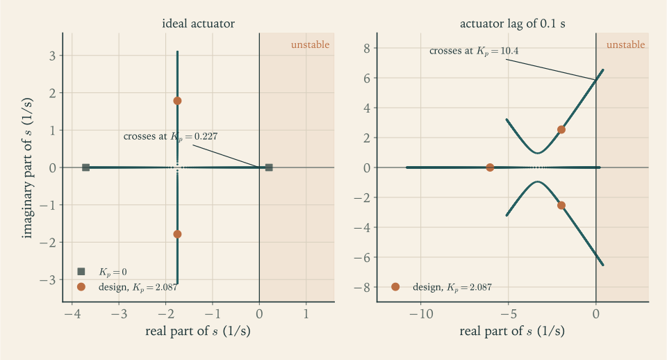
Roots. \(s=-1.75\pm1.79\,i\ \mathrm{s^{-1}}\) . An error decays as \(\exp(-1.75\,t)\) , losing a factor of ten every \(1.3\ \mathrm s\) .
What each gain is doing.
| Gains | Roots, \(\mathrm{s^{-1}}\) | Behaviour |
|---|---|---|
| \(K_p=0\) , \(K_d=0\) | \(+0.873\) , \(-0.873\) | diverges, doubling every \(0.79\ \mathrm s\) |
| \(K_p=0.1\) , \(K_d=1.042\ \mathrm s\) | \(+0.118\) , \(-3.618\) | still diverges: \(K_p\) is below \(M_\alpha/M_\delta=0.227\) |
| \(K_p=2.087\) , \(K_d=0\) | \(\pm2.5\,i\) | oscillates at \(2.5\ \mathrm{rad/s}\) for ever |
| \(K_p=2.087\) , \(K_d=1.042\ \mathrm s\) | \(-1.75\pm1.79\,i\) | decays |
Margins, read from the roots. The proportional gain could fall by a factor of \(2.087/0.227=9.2\) before the loop went unstable; equivalently, the aerodynamic moment could be \(9.2\) times larger than estimated. Given the uncertainty in \(M_\alpha\) admitted in Example 11.2, that is the margin that matters, and it is comfortable. Figure 11.2 shows how the roots move as \(K_p\) is raised from zero.
11.5 What the actuator cannot do
The feedback law assumed an engine that takes any angle instantly. A real actuator has a limit of travel and a finite speed, and each restricts the loop in a way that can be stated exactly.
Limited travel. Suppose \(\lvert\delta\rvert\le\delta_{\max}\) , and drop the wind. Write \(s_{\mathrm{div}}=\sqrt{M_\alpha/I_y}\) for the divergence rate, the positive root of the uncontrolled polynomial of Section 11.4, and consider the combination
the error rate plus \(s_{\mathrm{div}}\) times the error. Differentiating it and using the rotational equation \(I_y\,\mathrm d^2(\vartheta-\vartheta_{\mathrm{ref}})/\mathrm dt^2=M_\alpha(\vartheta-\vartheta_{\mathrm{ref}})+M_\delta\delta\) shows that it obeys a first-order equation of its own:
This is the unstable part of the motion, isolated. It grows at rate \(s_{\mathrm{div}}\) unless the gimbal term opposes it, and the gimbal term is bounded.
Proposition 11.3 (what a limited gimbal can recover). With \(\lvert\delta\rvert\le\delta_{\max}\) and no wind, the attitude error can be brought back to zero if and only if
Proof. Call the bracketed combination of the displayed equation \(Z\) , so that \(\dot Z=s_{\mathrm{div}}Z+(M_\delta/I_y)\delta\) . If \(\lvert Z\rvert\) exceeds \((M_\delta/I_y)\delta_{\max}/s_{\mathrm{div}}\) , then \(s_{\mathrm{div}}\lvert Z\rvert\) exceeds the largest value the gimbal term can take, \(\dot Z\) has the sign of \(Z\) for every admissible \(\delta\) , and \(\lvert Z\rvert\) grows without bound; the error cannot return to zero. If \(\lvert Z\rvert\) is smaller than that value, choosing \(\delta=-\delta_{\max}\) times the sign of \(Z\) makes \(\lvert Z\rvert\) decrease, and it reaches zero in finite time. Once \(Z=0\) the error obeys \(\mathrm d(\vartheta-\vartheta_{\mathrm{ref}})/\mathrm dt=-s_{\mathrm{div}}(\vartheta-\vartheta_{\mathrm{ref}})\) and decays, with the gimbal holding \(Z\) at zero, which needs \(\delta=0\) . Dividing the bound by \(s_{\mathrm{div}}\) and using \(s_{\mathrm{div}}^2=M_\alpha/I_y\) gives the stated form.
For an error with no rate the condition is \(\lvert\vartheta-\vartheta_{\mathrm{ref}}\rvert\) below \((M_\delta/M_\alpha)\delta_{\max}\) , the largest angle that can be trimmed. A nose already swinging outward counts against the limit, at \(1/s_{\mathrm{div}}\) seconds of rate per radian. An unstable vehicle with a bounded actuator has a boundary beyond which no control law can save it. Feedback gains do not appear in the proposition, because it is about what is possible, and the gains only choose among possible responses.
Limited speed. Let the engine angle follow its command with a first-order lag of time constant \(t_{\mathrm{act}}\) : \(t_{\mathrm{act}}\,\dot\delta=\delta_{\mathrm{cmd}}-\delta\) , where \(\delta_{\mathrm{cmd}}\) is the output of the feedback law. The closed loop is now third order. Eliminating \(\delta\) , its characteristic polynomial is
A cubic’s roots are awkward to write down, but whether they all have negative real parts can be read from its coefficients.
Proposition 11.4 (a cubic with all roots in the left half plane). The real polynomial \(s^3+\mathcal C_2s^2+\mathcal C_1s+\mathcal C_0\) has all three roots with negative real parts if and only if \(\mathcal C_2>0\) , \(\mathcal C_0>0\) , and \(\mathcal C_2\mathcal C_1>\mathcal C_0\) .
Proof. A real cubic has a real root; write the polynomial as \((s+\mathcal B_1)(s^2+\mathcal B_2s+\mathcal B_3)\) with real constants, so that \(\mathcal C_2=\mathcal B_1+\mathcal B_2\) , \(\mathcal C_1=\mathcal B_3+\mathcal B_1\mathcal B_2\) , \(\mathcal C_0=\mathcal B_1\mathcal B_3\) , and \(\mathcal C_2\mathcal C_1-\mathcal C_0=\mathcal B_2(\mathcal B_3+\mathcal B_1\mathcal C_2)\) . By the argument of Proposition 11.2 the roots all have negative real parts exactly when \(\mathcal B_1\) , \(\mathcal B_2\) , \(\mathcal B_3\) are all positive. If they are, the three conditions follow at once. Conversely, suppose the three conditions hold. Since \(\mathcal C_0=\mathcal B_1\mathcal B_3\) is positive, \(\mathcal B_1\) and \(\mathcal B_3\) have the same sign. If both were negative, \(\mathcal B_3+\mathcal B_1\mathcal C_2\) would be negative, so \(\mathcal C_2\mathcal C_1-\mathcal C_0>0\) would force \(\mathcal B_2<0\) , and then \(\mathcal C_2=\mathcal B_1+\mathcal B_2\) would be negative, a contradiction. So \(\mathcal B_1\) and \(\mathcal B_3\) are positive, \(\mathcal B_3+\mathcal B_1\mathcal C_2\) is positive, and \(\mathcal C_2\mathcal C_1-\mathcal C_0>0\) gives \(\mathcal B_2>0\) . (The constants \(\mathcal B_1\) , \(\mathcal B_2\) , \(\mathcal B_3\) appear in this proof only.)
Dividing the loop’s polynomial by \(t_{\mathrm{act}}I_y\) and applying the proposition, the first condition holds automatically, the second is \(K_p>M_\alpha/M_\delta\) as before, and the third, after the terms in \(M_\alpha\) cancel, is
The derivative gain must exceed the proportional gain times the actuator’s lag. Read the other way, for a given \(K_d\) the proportional gain has an upper limit, \(K_d/t_{\mathrm{act}}\) , as well as its lower limit \(M_\alpha/M_\delta\) . Too little gain and the air wins; too much and the lagging engine arrives late with a correction that has become a push in the wrong phase. A loop of this kind is called conditionally stable: it works only inside a window of gain.
Example 11.5: The actuator’s limits for the reference launcher
Travel. With \(\delta_{\max}=5^\circ\) (illustrative) and \(M_\delta/M_\alpha=1/0.227=4.41\) , the recoverable set at maximum dynamic pressure is
An error of \(10^\circ\) growing at \(12^\circ\) per second gives \(10+(1.146)(12)=23.8^\circ\) and is beyond recovery, although \(10^\circ\) at rest would be well inside.
Speed. With the gains of Example 11.4 the lag must satisfy \(t_{\mathrm{act}}<K_d/K_p=1.042/2.087=0.499\ \mathrm s\) . The roots of the cubic confirm it:
| Lag \(t_{\mathrm{act}}\) | Roots, \(\mathrm{s^{-1}}\) | |
|---|---|---|
| \(0.05\ \mathrm s\) | \(-16.2\) , \(-1.90\pm2.03\,i\) | close to the ideal \(-1.75\pm1.79\,i\) |
| \(0.1\ \mathrm s\) | \(-6.05\) , \(-1.98\pm2.54\,i\) | stable, faster and less damped |
| \(0.3\ \mathrm s\) | \(-2.40\) , \(-0.47\pm2.91\,i\) | stable, poorly damped |
| \(0.499\ \mathrm s\) | \(-2.00\) , \(\pm2.50\,i\) | on the boundary |
| \(0.6\ \mathrm s\) | \(-1.89\) , \(+0.11\pm2.34\,i\) | unstable |
For an actuator with \(t_{\mathrm{act}}=0.1\ \mathrm s\) (illustrative) the window of proportional gain, at this \(K_d\) , runs from \(0.227\) to \(1.042/0.1=10.4\) . The design value \(2.087\) sits a factor of \(9.2\) above the bottom and a factor of \(5.0\) below the top.
Proportional feedback alone, revisited. With \(K_d=0\) the condition \(K_d>t_{\mathrm{act}}K_p\) fails for every positive lag. The undamped oscillation of Example 11.4 was the best case; with any real actuator it grows. For \(t_{\mathrm{act}}=0.1\ \mathrm s\) the roots are \(-10.6\) and \(+0.31\pm2.41\,i\) .
11.6 Coefficients that will not stay still
The analysis so far froze the coefficients at one instant. In flight, dynamic pressure rises and falls, the thrust grows as the air thins, the centre of mass moves, and the inertia falls by a factor of three. Evaluating the same formulas along the reference ascent:
| Time | \(q\) | \(x_{\mathrm{cm}}\) | \(I_y\) | \(M_\alpha\) | \(M_\delta\) | \(\sqrt{M_\alpha/I_y}\) | \(M_\alpha/M_\delta\) |
|---|---|---|---|---|---|---|---|
| \(30\ \mathrm s\) | \(7.2\ \mathrm{kPa}\) | \(21.20\ \mathrm m\) | \(1.129\times10^{7}\) | \(1.74\times10^{6}\) | \(3.20\times10^{7}\) | \(0.393\ \mathrm{s^{-1}}\) | \(0.054\) |
| \(60\ \mathrm s\) | \(27.0\ \mathrm{kPa}\) | \(21.17\ \mathrm m\) | \(1.070\times10^{7}\) | \(6.55\times10^{6}\) | \(3.35\times10^{7}\) | \(0.782\ \mathrm{s^{-1}}\) | \(0.196\) |
| \(78.5\ \mathrm s\) | \(32.8\ \mathrm{kPa}\) | \(20.95\ \mathrm m\) | \(1.034\times10^{7}\) | \(7.87\times10^{6}\) | \(3.47\times10^{7}\) | \(0.873\ \mathrm{s^{-1}}\) | \(0.227\) |
| \(100\ \mathrm s\) | \(25.7\ \mathrm{kPa}\) | \(20.39\ \mathrm m\) | \(9.81\times10^{6}\) | \(5.95\times10^{6}\) | \(3.66\times10^{7}\) | \(0.779\ \mathrm{s^{-1}}\) | \(0.163\) |
| \(120\ \mathrm s\) | \(13.6\ \mathrm{kPa}\) | \(19.39\ \mathrm m\) | \(9.05\times10^{6}\) | \(2.96\times10^{6}\) | \(3.92\times10^{7}\) | \(0.572\ \mathrm{s^{-1}}\) | \(0.075\) |
| \(160\ \mathrm s\) | \(1.3\ \mathrm{kPa}\) | \(14.10\ \mathrm m\) | \(5.26\times10^{6}\) | \(1.83\times10^{5}\) | \(5.25\times10^{7}\) | \(0.187\ \mathrm{s^{-1}}\) | \(0.003\) |
Inertias are in \(\mathrm{kg\cdot m^2}\) and moments in \(\mathrm{N\cdot m/rad}\) . The instability follows the dynamic pressure and is worst, in both of the last two columns, within a few seconds of its peak. Late in the burn the air has gone, the centre of mass has moved forward so the engines have a longer arm, and the inertia has dropped: the engines’ authority per unit of inertia, \(M_\delta/I_y\) , triples.
Is a frozen analysis legitimate? Not as a theorem. A linear equation whose coefficients vary in time can be unstable even though every frozen version of it is stable; freezing is safe only when the coefficients change slowly compared with the motion being analysed. Here the loop settles in about two seconds and the coefficients change by tens of percent over twenty, so the approximation is reasonable, and Section 11.8 tests it by simulation, where nothing is frozen.
Example 11.6: One pair of gains for the whole burn, or a schedule
Fixed gains. Keep \(K_p=2.087\) and \(K_d=1.042\ \mathrm s\) throughout, and compute the frozen roots at each time from \(\omega_{\mathrm{nat}}^2=(M_\delta K_p-M_\alpha)/I_y\) and \(2\zeta_{\mathrm{damp}}\omega_{\mathrm{nat}}=M_\delta K_d/I_y\) :
| Time | \(\omega_{\mathrm{nat}}\) with fixed gains | \(\zeta_{\mathrm{damp}}\) with fixed gains | Scheduled \(K_p\) | Scheduled \(K_d\) |
|---|---|---|---|---|
| \(30\ \mathrm s\) | \(2.40\ \mathrm{rad/s}\) | \(0.62\) | \(2.259\) | \(1.235\ \mathrm s\) |
| \(78.5\ \mathrm s\) | \(2.50\ \mathrm{rad/s}\) | \(0.70\) | \(2.087\) | \(1.042\ \mathrm s\) |
| \(120\ \mathrm s\) | \(2.95\ \mathrm{rad/s}\) | \(0.76\) | \(1.518\) | \(0.808\ \mathrm s\) |
| \(160\ \mathrm s\) | \(4.56\ \mathrm{rad/s}\) | \(1.14\) | \(0.630\) | \(0.351\ \mathrm s\) |
The loop is stable at every instant with the fixed gains, and well damped. But its frequency drifts upward, nearly doubling by the end of the burn, as the same gimbal angles act on a lighter, shorter-coupled vehicle.
Scheduled gains. The last two columns are the gains that hold \(\omega_{\mathrm{nat}}=2.5\ \mathrm{rad/s}\) and \(\zeta_{\mathrm{damp}}=0.7\) at each time, from the formulas of Section 11.4. They fall by a factor of more than three across the burn. Changing the gains with time or with measured flight condition in this way is called gain scheduling. Whether the upward drift of the fixed-gain frequency matters depends on what else in the vehicle moves at a few radians per second, which is the subject of Section 11.9.
11.7 Why the frozen picture is not the whole loop
Three things were left out of the linear model besides the time variation, and the simulation includes all of them. The path responds: the normal force and the sideways component of the gimballed thrust both act on the centre of mass, so \(\theta\)
is not quite the planned \(\theta\)
. The engine has its travel limit. And the full trigonometry is kept. For a system that is differentiable near its reference motion, stability of the linearization with all roots in the left half plane implies that small disturbances of the full system decay; that is the theorem on stability by linearization in Differential Equations (math.differential-equations.linearization-stability), stated there for an equilibrium of a system with continuously differentiable right-hand side. The simulation shows how large “small” is.
11.8 Flying through the jet stream
The model. Revision A on the reference ascent of Example 7.6, from \(30\ \mathrm s\) to \(120\ \mathrm s\) , as a rigid body in the flight plane: the two translational equations of Chapter 7 with the thrust directed at the angle \(\vartheta-\delta\) , the normal force \(qSC_{N\alpha}\alpha\) added perpendicular to the axis, and drag along the relative wind; the rotational equation \(I_y\ddot\vartheta=M_\alpha\alpha+Fl_g\sin\delta\) ; mass, centre of mass, and inertia recomputed at every step from the layout of Example 11.1. The commanded attitude is the path angle of the planned, windless gravity turn, which is integrated alongside. The feedback law is that of Section 11.4 with the fixed gains of Example 11.4 and a \(5^\circ\) limit. Integration is by the Runge-Kutta method with steps of \(0.02\ \mathrm s\) .
Example 11.7: The controlled launcher in a wind
Still air. With no wind the controlled vehicle follows the planned path: the attitude error never exceeds \(0.003^\circ\) , the gimbal angle stays under \(0.01^\circ\) , and at \(120\ \mathrm s\) the position differs from the point-mass trajectory by \(1\ \mathrm m\) . A gravity turn asks almost nothing of the engines, because the commanded attitude is the one the vehicle’s own velocity already has. This is the check that the rigid-body program reduces to Chapter 7’s when it should.
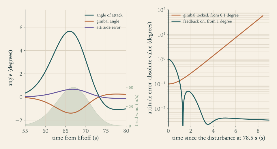
The uncontrolled vehicle. Start at \(78.5\ \mathrm s\) with an attitude error of \(0.1^\circ\) and the gimbal locked at zero:
| Time since release | \(1\ \mathrm s\) | \(2\ \mathrm s\) | \(4\ \mathrm s\) | \(6\ \mathrm s\) | \(8\ \mathrm s\) |
|---|---|---|---|---|---|
| Attitude error | \(0.14^\circ\) | \(0.27^\circ\) | \(1.39^\circ\) | \(7.5^\circ\) | \(40.5^\circ\) |
From \(2\ \mathrm s\) on, each second multiplies the error by about \(2.3\) , which is \(\exp(0.84)\) , close to the \(\exp(0.873)\) of Example 11.2. The first second is slower because the released vehicle starts with no error rate. By \(8.4\ \mathrm s\) the error has passed one radian.
A head wind. Let a wind blow against the direction of flight with speed \(50\exp\bigl[-((z-10\ \mathrm{km})/2\ \mathrm{km})^2\bigr]\ \mathrm{m/s}\) : the cited typical jet speed, in a layer of illustrative shape centred at \(10\ \mathrm{km}\) . The vehicle climbs through it between about \(58\) and \(74\ \mathrm s\) .
| Quantity | Peak value | Time |
|---|---|---|
| Angle of attack | \(5.66^\circ\) | \(66.0\ \mathrm s\) |
| Gimbal angle | \(-1.40^\circ\) | \(66.3\ \mathrm s\) |
| Attitude error | \(0.66^\circ\) | \(66.8\ \mathrm s\) |
| Load \(q\,\alpha\) | \(3.38\ \mathrm{kPa\cdot rad}\) | \(66.3\ \mathrm s\) |
Against the linear prediction. At the peak the wind is \(48.7\ \mathrm{m/s}\) , the airspeed \(418\ \mathrm{m/s}\) , and the dynamic pressure, raised by the head wind, \(34.1\ \mathrm{kPa}\) . The relative wind lies \(5.01^\circ\) below the planned path, and that is the \(\alpha_w\) of the linear model. It is less than the \(5.7^\circ\) of Example 11.3 because the path has responded: the normal force, \(47.6\ \mathrm{kN}\) , and the sideways component of the deflected thrust, \(59.0\ \mathrm{kN}\) , both push the vehicle the way the wind is blowing, upward and back across its path, and by the peak they have turned its velocity \(0.79^\circ\) more nearly vertical, toward the direction from which the relative wind arrives. With \(M_\alpha=(34\,103)(7.07)(2)(17.12)=8.26\times10^{6}\ \mathrm{N\cdot m/rad}\) and \(M_\delta=3.39\times10^{7}\ \mathrm{N\cdot m/rad}\) at that instant, the steady-state formulas of Section 11.4 give
and an attitude error of \(0.66^\circ\) . The simulation’s \(5.66^\circ\) , \(-1.40^\circ\) , and \(0.66^\circ\) agree: the wind changes slowly enough, over several seconds, that the loop is always close to its steady state.
What the wind did to the flight. The engines used \(1.4^\circ\) of their \(5^\circ\) . The attitude was held within two thirds of a degree. At \(120\ \mathrm s\) the vehicle is \(429\ \mathrm m\) and \(5.9\ \mathrm{m/s}\) from where the windless flight would have put it, an error that Chapter 10’s guidance removes on the second stage at a cost of a few metres per second. A tail wind of the same strength gives a peak angle of attack of \(-6.30^\circ\) and a gimbal angle of \(+1.22^\circ\) .
What breaks it. Three variations, each chosen to violate one of the conditions found above. With the gimbal limited to \(1^\circ\) , less than the \(1.4^\circ\) the wind demands, the engines saturate at \(63\ \mathrm s\) and the vehicle tumbles by \(69\ \mathrm s\) . With an actuator lag of \(0.6\ \mathrm s\) , above the limit of \(0.499\ \mathrm s\) , a \(0.1^\circ\) disturbance at \(30\ \mathrm s\) grows into a tumble by \(77.5\ \mathrm s\) in still air. With proportional feedback alone and a lag of \(0.1\ \mathrm s\) , the same disturbance tumbles the vehicle by \(57\ \mathrm s\) . With the design gains and the \(0.1\ \mathrm s\) lag, the wind case is indistinguishable from the table above. Figure 11.3 shows the wind response and the uncontrolled divergence.
The number the structure cares about. The peak of \(q\,\alpha\) , \(3.4\ \mathrm{kPa\cdot rad}\) , is the sideways load indicator of Section 7.7. It corresponds to a normal force of \((3378\ \mathrm{Pa})(7.07\ \mathrm{m^2})(2)=47.8\ \mathrm{kN}\) on the nose, with an opposing force at the gimbal, bending the vehicle about its middle. This load, not the gimbal travel, is what a wind really threatens, and it is larger than anything Example 10.8 considered planning for. Holding attitude does nothing to reduce it; the feedback law of this chapter keeps the vehicle pointed and lets the wind load it.
11.9 What the rigid model omits
The roots in Example 11.4 could have been placed anywhere. Why \(2.5\ \mathrm{rad/s}\) , and not \(25\) , which would hold the attitude ten times more tightly? The rigid-body analysis offers no objection: with an ideal actuator, Proposition 11.2 is satisfied by any gains above the minimum. The objection comes from three motions the model does not contain, each of which behaves like a lightly damped oscillator attached to the pitch equation.
Slosh. The propellant is liquid with a free surface, and the surface can swing from side to side like water carried in a pan. To the vehicle it looks like a pendulum hung inside each tank. For an upright cylindrical tank of radius \(R_{\mathrm{tank}}\) , filled to depth \(d_{\mathrm{liq}}\) , under an acceleration \(F/m\) along the axis, the frequency of the first sideways mode is
(NASA SP-8009; see sources). The formula is quoted, not derived; the constant \(1.841\) is the first root of the derivative of a Bessel function, and the mathematics is separation of variables for Laplace’s equation in a cylinder. For depths greater than the radius the hyperbolic tangent is nearly \(1\) and the liquid swings as a pendulum of length \(R_{\mathrm{tank}}/1.841\) . The same source notes that the damping from the liquid’s wiping against smooth walls is generally not adequate, and that baffles are added to supply the damping needed to prevent instabilities in the closed-loop control system.
Bending. The structure is a long thin tube and it flexes. In its first bending mode the nose and tail move one way while the middle moves the other. An attitude sensor mounted on the structure measures the local slope, which includes the bending, and reports it to the feedback law as if it were rigid rotation.
The engine’s own inertia. A swivelling engine is a mass on the end of the vehicle, and accelerating it sideways pushes the vehicle the other way.
Each of these is excited by gimbal motion and each is sensed by the attitude instruments, so each closes a loop of its own through the feedback law. If the rigid loop’s frequency is raised toward one of them, the law responds to the mode’s motion with a phase that can feed energy into it. The rigid analysis cannot see this, because the polynomial it tests does not contain the mode. The working rule is separation of frequencies: keep the rigid-body loop well below the lowest of the unmodelled modes, or shape the feedback so that it does not respond at their frequencies. Designing those shapes, and the structure and baffles they depend on, is outside this course.
Example 11.8: How close the slosh is
At maximum dynamic pressure. The acceleration along the axis is the thrust less the drag over the mass, \((2461.6-69.6)/114.14=20.96\ \mathrm{m/s^2}\) . The oxygen tank is filled to \((0.5353)(11.84)=6.34\ \mathrm m\) , more than four radii, so the hyperbolic tangent is \(1\) and
or \(0.81\) cycles per second. The kerosene tank has the same radius, is filled to \(3.9\ \mathrm m\) , and gives the same value.
Compared with the loop. The attitude loop at \(2.5\ \mathrm{rad/s}\) is a factor of two below the slosh frequency. That is a thin separation, and it is the reason the frequency was not chosen higher. It is also why the upward drift of Example 11.6 matters: with fixed gains the loop reaches \(4.6\ \mathrm{rad/s}\) by \(160\ \mathrm s\) . The slosh frequency rises too, since the acceleration grows as the vehicle lightens, but the tanks are then nearly empty and the comparison has to be made at each instant (Exercise 17). Scheduling the gains keeps the loop at \(2.5\ \mathrm{rad/s}\) and the separation growing.
Common mistake. Concluding from Proposition 11.2 that raising both gains is always safe. The proposition is a statement about a model with one degree of rotational freedom and a perfect actuator. Proposition 11.4 already showed that one extra first-order element creates an upper limit on the proportional gain for a given derivative gain. Every unmodelled mode creates another.
11.10 The reference launcher after this chapter
Every number in this table is for Revision A on the reference ascent of Example 7.6; Section 12.9 repeats the principal ones for Revision C.
| Item | Value | Basis |
|---|---|---|
| Length and layout | \(36.56\ \mathrm m\) ; stations of Example 11.1 | Chapter 6 lengths, illustrative arrangement |
| Centre of mass at maximum dynamic pressure | \(20.95\ \mathrm m\) from the nose | mass model of Example 11.1 |
| Pitch moment of inertia there | \(1.034\times10^{7}\ \mathrm{kg\cdot m^2}\) | same |
| Centre of pressure | \(4.0\ \mathrm m\) from the nose; \(16.95\ \mathrm m\) ahead of the centre of mass | slender-body theory, conical fairing |
| Aerodynamic moment \(M_\alpha\) | \(7.87\times10^{6}\ \mathrm{N\cdot m/rad}\) ; divergence doubles in \(0.79\ \mathrm s\) | Example 11.2 |
| Control moment \(M_\delta\) | \(3.47\times10^{7}\ \mathrm{N\cdot m/rad}\) ; \(0.227^\circ\) of gimbal per degree of angle of attack | Example 11.3 |
| Feedback gains at maximum dynamic pressure | \(K_p=2.087\) , \(K_d=1.042\ \mathrm s\) ; roots \(-1.75\pm1.79\,i\ \mathrm{s^{-1}}\) | Example 11.4 |
| Gain window with a \(0.1\ \mathrm s\) actuator | \(0.227<K_p<10.4\) | Example 11.5 |
| Gimbal travel used in a \(50\ \mathrm{m/s}\) jet | \(1.4^\circ\) of an assumed \(5^\circ\) | Example 11.7 |
| Peak load in that wind | \(q\,\alpha=3.4\ \mathrm{kPa\cdot rad}\) ; \(47.8\ \mathrm{kN}\) on the nose | Example 11.7 |
| Lowest slosh frequency at maximum dynamic pressure | \(5.07\ \mathrm{rad/s}\) , twice the loop’s | Example 11.8 |
The vehicle can be controlled. A statically unstable body with a divergence time of about a second is held within a degree of its commanded attitude, through a strong wind, by engine deflections of a degree and a half, with a feedback law of two gains. The margins on the rigid-body model are wide: a factor of nine on the aerodynamic moment, a factor of five on the gain’s upper side, a factor of three and a half on gimbal travel.
No mass or budget number changes. Two items are passed to the design review of Chapter 12. The first is the wind load: \(3.4\ \mathrm{kPa\cdot rad}\) at \(34\ \mathrm{kPa}\) is a bending load that the mass estimate of Chapter 6 never examined, its tank walls having been sized for internal pressure with a factor of two for everything else. The second is the frequency separation, a factor of two between the attitude loop and the propellant slosh on a rigid-body model with a guessed layout. Neither can be closed with the tools of this course, and both are of the kind that changes a structure’s mass.
Where this chapter’s model stops being accurate. The aerodynamic coefficients are slender-body estimates. The body is rigid and its propellant frozen in place. Sensors are perfect and the actuator, at most, a first-order lag. Only pitch was treated; yaw is the same problem in the perpendicular plane and roll is a separate one. And the feedback law holds attitude without regard to load, where real vehicles also steer to reduce the angle of attack in a wind. What survives all of these is the structure of the problem: an unstable second-order plant, a control moment from the far end of the vehicle, a window of gain bounded below by the air and above by everything that lags or flexes.
With the vehicle shown to be steerable along the path that Chapter 10 chose, every phase of the launch has now been modelled. One piece of hardware is still in orbit with no account of where it goes: the spent upper stage, on its way down from \(400\ \mathrm{km}\) .
Exercises
-
Define the pitch attitude, the angle of attack, the gimbal angle, the centre of mass, and the centre of pressure, stating the sign convention of each angle and the end from which stations are measured. Then state the condition for static stability in terms of the two stations and explain it with the arrow of Section 11.2.
Hint
Pitch attitude and path angle are measured from the local horizontal, the angle of attack from the air-relative velocity to the axis, positive nose-up; the gimbal angle is positive when its moment raises the nose. Stations are measured from the nose tip. Stable means the centre of pressure has the larger station. For the arrow, say where its mass is and where its feathers put the air’s force.
-
A simplified vehicle consists of three uniform segments along its axis: \(6000\ \mathrm{kg}\) from station \(0\) to \(8\ \mathrm m\) , \(20\,000\ \mathrm{kg}\) from \(8\) to \(20\ \mathrm m\) , and \(74\,000\ \mathrm{kg}\) from \(20\) to \(32\ \mathrm m\) (illustrative values). Compute its centre of mass and its pitch moment of inertia about the centre of mass, and compare the inertia with that of a uniform rod of the same mass and length.
Solution
Centre of mass. The segment centres are at \(4\) , \(14\) , and \(26\ \mathrm m\) , and the total mass is \(100\,000\ \mathrm{kg}\) :
\[ x_{\mathrm{cm}}=\frac{(6000)(4)+(20\,000)(14)+(74\,000)(26)}{100\,000}=22.28\ \mathrm m . \]Inertia. Each segment contributes \(m(l^2/12+d^2)\) with \(d\) the distance of its centre from \(22.28\ \mathrm m\) :
\[ I_y=6000\Bigl(\frac{8^2}{12}+18.28^2\Bigr)+20\,000\Bigl(\frac{12^2}{12}+8.28^2\Bigr)+74\,000\Bigl(\frac{12^2}{12}+3.72^2\Bigr)=5.56\times10^{6}\ \mathrm{kg\cdot m^2}. \]Comparison. A uniform rod of \(100\,000\ \mathrm{kg}\) and \(32\ \mathrm m\) has \(mL^2/12=8.53\times10^{6}\ \mathrm{kg\cdot m^2}\) . The vehicle has \(65\) percent of that, because three quarters of its mass is in the rear segment, close to the centre of mass. Concentrating mass near the centre lowers the inertia, which makes the body easier to turn, for the engines and for the air alike.
-
From the definition \(I_y=\sum m_i\lvert\mathbf r_i\rvert^2\) : (a) show by integration that a uniform rod of mass \(m\) and length \(l\) has moment of inertia \(ml^2/12\) about its centre; (b) prove that the moment of inertia of any body about an axis at distance \(d\) from its centre of mass equals its moment of inertia about the centre of mass plus \(md^2\) ; (c) use (b) to justify the sum used in Example 11.1.
Hint
(a) Integrate \(x^2\,(m/l)\,\mathrm dx\) from \(-l/2\) to \(l/2\) . (b) Write each particle’s position from the new axis as the position from the centre of mass plus a fixed offset of length \(d\) , expand the square, and use \(\sum m_i\mathbf r_i=0\) to remove the cross term. (c) Apply (b) to each uniform segment, with (a) for its own inertia.
-
Use Proposition 11.1 to locate the centre of pressure of three noses of length \(l_n\) and base area \(S\) : (a) a cone; (b) a paraboloid whose cross-sectional area grows linearly with distance from the tip; (c) a blunt nose whose area reaches \(S\) within the first tenth of its length and is constant thereafter. Then explain what the proposition predicts for a section whose area decreases toward the rear.
Solution
Proposition 11.1 gives \(x_{\mathrm{cp}}=l_n-(\text{volume})/S\) .
(a) A cone has volume \(Sl_n/3\) , so \(x_{\mathrm{cp}}=\tfrac23l_n\) .
(b) If the area grows linearly, \(A=S\,x/l_n\) , the volume is \(Sl_n/2\) and \(x_{\mathrm{cp}}=\tfrac12l_n\) . Equivalently, \(\mathrm dA/\mathrm dx\) is constant, so the normal force is spread uniformly along the nose and acts at its middle.
(c) The area reaches \(S\) within the first tenth of the length, so \(\mathrm dA/\mathrm dx\) vanishes beyond it and all of the force is generated within that tenth: \(x_{\mathrm{cp}}\) lies between \(0\) and \(0.1\,l_n\) . The total force is unchanged, since \(C_{N\alpha}=2\) for any nose; a blunter nose moves the same force forward.
A section whose area decreases. There \(\mathrm dA/\mathrm dx\) is negative and so is the local normal force: a boat-tail is pushed in the direction opposite to the nose. Being at the rear, behind the centre of mass, a negative force there produces a nose-raising moment for a nose-up angle of attack, the same sense as the nose’s own. A narrowing tail is destabilizing; a widening one, a flare, is stabilizing.
-
Using the table of Section 11.6, compute the time for an uncontrolled disturbance to double at \(30\ \mathrm s\) , \(78.5\ \mathrm s\) , and \(120\ \mathrm s\) , and the gimbal angle needed to trim an angle of attack of \(3^\circ\) at each of those times. At which time is the vehicle hardest to control, and why is it not the time of greatest thrust?
Solution
The doubling time is \(\ln2/\sqrt{M_\alpha/I_y}\) and the trim angle is \((M_\alpha/M_\delta)\alpha\) .
Time \(\sqrt{M_\alpha/I_y}\) Doubling time Gimbal to trim \(3^\circ\) \(30\ \mathrm s\) \(0.393\ \mathrm{s^{-1}}\) \(1.76\ \mathrm s\) \(0.16^\circ\) \(78.5\ \mathrm s\) \(0.873\ \mathrm{s^{-1}}\) \(0.79\ \mathrm s\) \(0.68^\circ\) \(120\ \mathrm s\) \(0.572\ \mathrm{s^{-1}}\) \(1.21\ \mathrm s\) \(0.23^\circ\) The vehicle is hardest to control at maximum dynamic pressure: the divergence is fastest and each degree of angle of attack claims the most gimbal. The reason is that \(M_\alpha\) is proportional to \(q\) , which peaks there, while the lever arm and the inertia change little. Thrust is greatest later, in near vacuum, but thrust is on the controlling side of the ledger: more thrust means more \(M_\delta\) . The difficulty comes from the air, and by the time the thrust has peaked the air has gone.
-
A student explains: “The launch vehicle is unstable because it is so heavy. Model rockets are light, so the air can straighten them out.” (a) Identify the error, using the definition of static stability. (b) Show from the rotational equation that making the vehicle heavier, with the same shape and mass distribution, slows the divergence instead of causing it. (c) Using Example 11.2, state what fins would have to do and give two reasons launch vehicles omit them.
Solution
(a) Static stability depends on where the normal force acts relative to the centre of mass, not on how large the mass is. The launch vehicle is unstable because its normal force is generated on the nose, \(17\ \mathrm m\) ahead of its centre of mass. A model rocket is stable because its fins generate a larger normal force at the tail, putting the centre of pressure behind the centre of mass.
(b) The divergence rate is \(\sqrt{M_\alpha/I_y}\) . Scaling every mass by the same factor leaves the centre of mass, and hence \(M_\alpha\) , unchanged and multiplies \(I_y\) by that factor, so a heavier vehicle of the same shape diverges more slowly.
(c) By Example 11.2, fins at the tail would have to supply a normal-force slope of \(2.90\) , one and a half times the nose’s, to move the centre of pressure \(2\ \mathrm m\) behind the centre of mass. Launch vehicles omit them because fins of that size cost mass and drag on the first stage, and because they do nothing at liftoff, where the dynamic pressure is zero, or above the atmosphere; the engines must be able to steer in those phases anyway.
-
At maximum dynamic pressure the reference launcher holds a steady angle of attack of \(2^\circ\) . (a) Find the gimbal angle. (b) Compute the normal force, the sideways component of the thrust, and their sum, giving the direction of each relative to the nose. (c) Compute the resulting acceleration of the centre of mass perpendicular to the axis and the rate at which it turns a velocity of \(542\ \mathrm{m/s}\) .
Solution
(a) \(\delta=-(M_\alpha/M_\delta)\alpha=-(0.227)(2^\circ)=-0.45^\circ\) : the engines are deflected to push the nose down against the air.
(b) The normal force is \(qSC_{N\alpha}\alpha=(32\,832)(7.07)(2)(0.03491)=16.2\ \mathrm{kN}\) , directed perpendicular to the axis toward the side to which the nose is raised. The thrust’s sideways component is \(F\sin\lvert\delta\rvert=(2.4616\times10^{6})\sin0.453^\circ=19.5\ \mathrm{kN}\) . A gimbal angle that lowers the nose pushes the tail, and so the vehicle, toward that same side. The two add: \(35.7\ \mathrm{kN}\) .
(c) \(35\,670\ \mathrm N/114\,143\ \mathrm{kg}=0.3125\ \mathrm{m/s^2}\) perpendicular to the axis, which turns a velocity of \(542\ \mathrm{m/s}\) at \(0.3125/542=5.8\times10^{-4}\ \mathrm{rad/s}\) , or \(0.033^\circ\) per second. In trim the moments cancel but the forces do not, and both push the vehicle toward the side to which its nose is raised above the relative wind. In Example 11.7 the wind is a head wind, that side is upward and downwind, and the velocity had turned \(0.79^\circ\) more nearly vertical by the time of the peak.
-
For the coefficients of the reference launcher at maximum dynamic pressure, find the gains that give \(\omega_{\mathrm{nat}}=2.0\ \mathrm{rad/s}\) and \(\zeta_{\mathrm{damp}}=0.5\) , the roots, and the time for an error to fall to one percent of its initial size. Compare the proportional gain’s margin above \(M_\alpha/M_\delta\) with that of Example 11.4.
Solution
With \(I_y=1.0336\times10^{7}\) , \(M_\alpha=7.869\times10^{6}\) , and \(M_\delta=3.473\times10^{7}\) in SI units,
\[ K_p=\frac{(1.0336\times10^{7})(2.0)^2+7.869\times10^{6}}{3.473\times10^{7}}=1.417,\qquad K_d=\frac{2(0.5)(2.0)(1.0336\times10^{7})}{3.473\times10^{7}}=0.595\ \mathrm s . \]The roots are \(-\zeta_{\mathrm{damp}}\omega_{\mathrm{nat}}\pm i\,\omega_{\mathrm{nat}}\sqrt{1-\zeta_{\mathrm{damp}}^2}=-1.00\pm1.73\,i\ \mathrm{s^{-1}}\) . The envelope \(\exp(-t)\) falls to one percent at \(t=\ln100=4.6\ \mathrm s\) , against \(\ln100/1.75=2.6\ \mathrm s\) for the gains of Example 11.4. The proportional gain is \(1.417/0.227=6.3\) times its lower limit, where Example 11.4 had \(9.2\) : a slower loop is closer to the aerodynamic boundary, because the gimbal moment it commands per degree of error is smaller.
-
Prove directly, without quoting Proposition 11.2, that if \(M_\delta K_p<M_\alpha\) the closed-loop characteristic polynomial has a positive real root for every value of \(K_d\) . Interpret the result: why can no amount of rate feedback substitute for sufficient attitude feedback?
Solution
Let \(P(s)=I_ys^2+M_\delta K_ds+(M_\delta K_p-M_\alpha)\) with \(M_\delta K_p<M_\alpha\) . Then \(P(0)\) is negative. For large positive \(s\) the term \(I_ys^2\) dominates and \(P(s)\) is positive. A polynomial is continuous, so by the intermediate value theorem \(P\) vanishes at some positive \(s\) , whatever the value of \(K_d\) . That root gives a solution \(\exp(st)\) that grows.
Interpretation. The derivative term produces a moment only while the vehicle is rotating. With the vehicle momentarily at rest at a small error, the only moments are the air’s, \(M_\alpha\) per radian outward, and the proportional term’s, \(M_\delta K_p\) per radian inward. If the air’s is larger, the vehicle starts to move outward, and rate feedback can slow the departure but cannot reverse it, since reversing would require an inward moment at zero rate. Attitude feedback supplies the stiffness; rate feedback supplies only damping.
-
With \(K_d=0\) and an ideal actuator the closed loop is \(I_y\ddot\vartheta_{\mathrm{err}}+(M_\delta K_p-M_\alpha)\vartheta_{\mathrm{err}}=0\) for the error \(\vartheta_{\mathrm{err}}=\vartheta-\vartheta_{\mathrm{ref}}\) about a constant reference. (a) Show that the quantity \(\tfrac12I_y\dot\vartheta_{\mathrm{err}}^2+\tfrac12(M_\delta K_p-M_\alpha)\vartheta_{\mathrm{err}}^2\) is constant. (b) Deduce that the error neither grows nor decays. (c) Using Proposition 11.4, show that with any actuator lag the same loop is unstable, and explain in words where the energy comes from.
Solution
(a) Differentiate: \(I_y\dot\vartheta_{\mathrm{err}}\ddot\vartheta_{\mathrm{err}}+(M_\delta K_p-M_\alpha)\vartheta_{\mathrm{err}}\dot\vartheta_{\mathrm{err}}=\dot\vartheta_{\mathrm{err}}\,[I_y\ddot\vartheta_{\mathrm{err}}+(M_\delta K_p-M_\alpha)\vartheta_{\mathrm{err}}]=0\) by the equation of motion.
(b) With \(M_\delta K_p>M_\alpha\) both terms of the conserved quantity are nonnegative, so the motion stays on a closed curve in the plane of \(\vartheta_{\mathrm{err}}\) and \(\dot\vartheta_{\mathrm{err}}\) , an ellipse. The error can never exceed its largest initial excursion and can never settle to zero: it oscillates at \(\sqrt{(M_\delta K_p-M_\alpha)/I_y}\) for ever.
(c) With a lag the loop’s polynomial, divided by \(t_{\mathrm{act}}I_y\) , has \(\mathcal C_2=1/t_{\mathrm{act}}\) , \(\mathcal C_1=(M_\delta K_d-t_{\mathrm{act}}M_\alpha)/(t_{\mathrm{act}}I_y)\) , and \(\mathcal C_0=(M_\delta K_p-M_\alpha)/(t_{\mathrm{act}}I_y)\) , and Proposition 11.4’s third condition reduces to \(K_d>t_{\mathrm{act}}K_p\) . With \(K_d=0\) it fails for every positive \(t_{\mathrm{act}}\) , so some root has a nonnegative real part, and Example 11.5 shows it is positive. The energy comes from the engines. A lagging gimbal delivers its restoring moment late, so part of it acts in the direction of the motion instead of against the displacement, and over each cycle the gimbal moment does net positive work on the oscillation.
-
Apply Proposition 11.4 to the polynomial \(t_{\mathrm{act}}I_ys^3+I_ys^2+(M_\delta K_d-t_{\mathrm{act}}M_\alpha)s+(M_\delta K_p-M_\alpha)\) and derive the two conditions \(K_p>M_\alpha/M_\delta\) and \(K_d>t_{\mathrm{act}}K_p\) , showing each step. Then, for the gains of Example 11.4, find the largest proportional gain allowed when \(t_{\mathrm{act}}=0.2\ \mathrm s\) and the factor by which it exceeds the design value.
Solution
Divide the polynomial by \(t_{\mathrm{act}}I_y\) :
\[ \mathcal C_2=\frac1{t_{\mathrm{act}}},\qquad \mathcal C_1=\frac{M_\delta K_d-t_{\mathrm{act}}M_\alpha}{t_{\mathrm{act}}I_y},\qquad \mathcal C_0=\frac{M_\delta K_p-M_\alpha}{t_{\mathrm{act}}I_y}. \]The condition \(\mathcal C_2>0\) holds. The condition \(\mathcal C_0>0\) is \(K_p>M_\alpha/M_\delta\) . The condition \(\mathcal C_2\mathcal C_1>\mathcal C_0\) is
\[ \frac{M_\delta K_d-t_{\mathrm{act}}M_\alpha}{t_{\mathrm{act}}^2I_y}>\frac{M_\delta K_p-M_\alpha}{t_{\mathrm{act}}I_y} \quad\Longleftrightarrow\quad M_\delta K_d-t_{\mathrm{act}}M_\alpha>t_{\mathrm{act}}M_\delta K_p-t_{\mathrm{act}}M_\alpha , \]and the terms in \(M_\alpha\) cancel, leaving \(K_d>t_{\mathrm{act}}K_p\) .
For \(K_d=1.042\ \mathrm s\) and \(t_{\mathrm{act}}=0.2\ \mathrm s\) the largest proportional gain is \(1.042/0.2=5.21\) , which is \(5.21/2.087=2.5\) times the design value. Doubling the lag from \(0.1\) to \(0.2\ \mathrm s\) halves the upper margin from \(5.0\) to \(2.5\) .
-
The engines of the reference launcher are limited to \(3^\circ\) of gimbal. Using Proposition 11.3 at maximum dynamic pressure: (a) find the largest attitude error, with no rate, from which recovery is possible; (b) decide whether an error of \(5^\circ\) increasing at \(8^\circ\) per second can be recovered; (c) decide the same for an error of \(12^\circ\) decreasing at \(4^\circ\) per second; (d) explain why the feedback gains do not appear in your answers.
Solution
With \(M_\delta/M_\alpha=4.41\) and \(1/s_{\mathrm{div}}=1.146\ \mathrm s\) the recoverable set is \(\lvert\text{error}+(1.146\ \mathrm s)\,\text{rate}\rvert<(4.41)(3^\circ)=13.2^\circ\) .
(a) With no rate, errors up to \(13.2^\circ\) .
(b) \(5+(1.146)(8)=14.2^\circ\) , which exceeds \(13.2^\circ\) : not recoverable, although the error itself is small. The outward rate carries the vehicle past the trim limit before the engines can stop it.
(c) \(12+(1.146)(-4)=7.4^\circ\) , inside the bound: recoverable. The inward rate counts in the vehicle’s favour.
(d) The proposition describes which states can be recovered by some admissible gimbal history. The gains select one history, and cannot enlarge the set; a poor choice of gains can only fail to recover states that lie inside it.
-
(Computation.) Integrate the linear closed-loop equation of Section 11.4 with the coefficients and gains of Example 11.4 for a wind contribution \(\alpha_w\) that steps from zero to \(3^\circ\) at \(t=0\) , from rest. Report the peak and final values of the attitude error, the angle of attack, and the gimbal angle, and compare the final values with the steady-state formulas.
Answer
Final values: attitude error \(0.365^\circ\) , angle of attack \(3.365^\circ\) , gimbal \(-0.763^\circ\) , in agreement with the steady-state formulas. Peaks: error \(0.382^\circ\) and angle of attack \(3.382^\circ\) , an overshoot of \(4.6\) percent of the final error, as a damping ratio of \(0.7\) gives; gimbal \(-0.891^\circ\) .
-
Derive the three steady-state formulas of Section 11.4 for a constant wind contribution \(\alpha_w\) . Then show that the steady angle of attack exceeds \(\alpha_w\) by the factor \(1/(1-M_\alpha/(M_\delta K_p))\) , evaluate the factor for the gains of Example 11.4, and say what happens to it as \(K_p\) approaches its lower limit.
Solution
Set all derivatives to zero in the closed-loop equation: \((M_\delta K_p-M_\alpha)(\vartheta-\vartheta_{\mathrm{ref}})=M_\alpha\alpha_w\) , which is the first formula. The angle of attack is the error plus \(\alpha_w\) :
\[ \alpha=\alpha_w\Bigl(1+\frac{M_\alpha}{M_\delta K_p-M_\alpha}\Bigr)=\frac{M_\delta K_p}{M_\delta K_p-M_\alpha}\,\alpha_w . \]The gimbal angle is \(-K_p\) times the error, \(-K_pM_\alpha\alpha_w/(M_\delta K_p-M_\alpha)\) , which equals \(-(M_\alpha/M_\delta)\alpha\) on substituting the expression for \(\alpha\) .
Dividing numerator and denominator by \(M_\delta K_p\) gives the factor \(1/(1-M_\alpha/(M_\delta K_p))\) . For the gains of Example 11.4, \(M_\alpha/(M_\delta K_p)=0.227/2.087=0.109\) and the factor is \(1.122\) . As \(K_p\) falls toward \(M_\alpha/M_\delta\) the denominator goes to zero and the factor grows without bound: near the stability boundary the loop needs an enormous error to generate the trim deflection, which is another way of seeing that the boundary is a boundary.
-
Using the table of Section 11.6 and the fixed gains of Example 11.4, verify the entries of Example 11.6 at \(120\ \mathrm s\) : compute \(\omega_{\mathrm{nat}}\) and \(\zeta_{\mathrm{damp}}\) , and then the scheduled gains that restore \(2.5\ \mathrm{rad/s}\) and \(0.7\) . Explain which of the three changing quantities, \(I_y\) , \(M_\alpha\) , or \(M_\delta\) , is most responsible for the drift.
Answer
At \(120\ \mathrm s\) : \(\omega_{\mathrm{nat}}=\sqrt{[(3.92\times10^{7})(2.087)-2.96\times10^{6}]/9.05\times10^{6}}=2.95\ \mathrm{rad/s}\) and \(\zeta_{\mathrm{damp}}=0.76\) ; scheduled gains \(K_p=1.518\) and \(K_d=0.808\ \mathrm s\) . The drift comes mainly from \(M_\delta/I_y\) , which rises from \(3.36\) to \(4.33\ \mathrm{s^{-2}}\) as the inertia falls and the lever arm and thrust grow; the fall of \(M_\alpha/I_y\) from \(0.76\) to \(0.33\ \mathrm{s^{-2}}\) adds a little.
-
(Computation.) Write a rigid-body simulation of the reference launcher from \(30\) to \(120\ \mathrm s\) as described in Section 11.8, with the mass model of Example 11.1 and the wind of Example 11.7. Reproduce the four peak values of that example. Then double the wind speed and report the peak angle of attack, gimbal angle, and load, and say whether the vehicle remains controlled with \(5^\circ\) of gimbal.
Answer
With the wind doubled to \(100\ \mathrm{m/s}\) : peak angle of attack \(10.8^\circ\) , gimbal \(-3.0^\circ\) , attitude error \(1.4^\circ\) , load \(7.3\ \mathrm{kPa\cdot rad}\) . The vehicle remains controlled, with \(2^\circ\) of gimbal in hand, but the load has more than doubled, since the head wind also raises the dynamic pressure.
-
At \(160\ \mathrm s\) the reference launcher’s mass is \(48\,040\ \mathrm{kg}\) , its thrust \(2505\ \mathrm{kN}\) , drag is negligible, and \(5.3\) percent of the first stage’s propellant remains, so the oxygen tank is filled to \(0.63\ \mathrm m\) . (a) Compute the slosh frequency from the formula of Section 11.9, keeping the hyperbolic tangent. (b) Compare it with the fixed-gain loop frequency of \(4.56\ \mathrm{rad/s}\) at that time and with the scheduled \(2.5\ \mathrm{rad/s}\) . (c) Explain why the mass of liquid taking part in the slosh matters as well as its frequency.
Solution
(a) The acceleration is \(2.505\times10^{6}/48\,040=52.1\ \mathrm{m/s^2}\) . The depth is less than the radius, so the hyperbolic tangent matters: \(\tanh(1.841\times0.63/1.5)=\tanh0.773=0.649\) .
\[ \omega_{\mathrm{slosh}}=\sqrt{\frac{(1.841)(52.1)}{1.5}\,(0.649)}=6.44\ \mathrm{rad/s}. \](b) The fixed-gain loop at \(4.56\ \mathrm{rad/s}\) is a factor of \(1.4\) below it; the scheduled loop at \(2.5\ \mathrm{rad/s}\) is a factor of \(2.6\) below. With fixed gains the separation has shrunk from \(2.0\) at maximum dynamic pressure; with scheduled gains it has grown.
(c) The strength of the coupling depends on how much liquid moves. At \(160\ \mathrm s\) only \(5\) percent of the propellant is left, about \(5\ \mathrm t\) of oxygen in a vehicle of \(48\ \mathrm t\) , and in a shallow pool most of what remains takes part in the motion; at maximum dynamic pressure \(51\ \mathrm t\) of oxygen is present but only the upper part of a deep column sloshes. A mode with little mass in it disturbs the vehicle little, even at an awkward frequency. A full treatment needs the sloshing mass as well as the frequency, which the cited source tabulates.
-
This exercise uses Chapter 10. At ignition the second stage and payload have mass \(32\,045\ \mathrm{kg}\) , centre of mass at station \(7.24\ \mathrm m\) , and pitch inertia \(1.03\times10^{5}\ \mathrm{kg\cdot m^2}\) ; the engine gives \(282.8\ \mathrm{kN}\) and its gimbal is at station \(10.47\ \mathrm m\) , with \(5^\circ\) of travel (illustrative). There is no air. (a) Compute \(M_\delta\) and the largest angular acceleration. (b) Find the least time in which the stage can rotate through the \(6.8^\circ\) that Example 10.7 commands at staging, starting and ending at rest, and describe the gimbal history that achieves it. (c) State which result of Chapter 10 or of the cited optimal-control course tells you the form of that history. (d) Is the delay significant for the steering law?
Solution
(a) The arm is \(10.47-7.24=3.23\ \mathrm m\) , so \(M_\delta=(2.828\times10^{5})(3.23)=9.13\times10^{5}\ \mathrm{N\cdot m/rad}\) . With no air \(M_\alpha=0\) , and the largest angular acceleration, at \(\delta=5^\circ\) , is
\[ \frac{M_\delta\sin5^\circ}{I_y}=\frac{(9.13\times10^{5})(0.0872)}{1.03\times10^{5}}=0.773\ \mathrm{rad/s^2}. \](b) The fastest rest-to-rest rotation accelerates at the maximum for half the angle and decelerates at the maximum for the other half. Each half takes \(\sqrt{(6.8^\circ)(\pi/180^\circ)/0.773}=0.392\ \mathrm s\) , so the least time is \(0.78\ \mathrm s\) : full gimbal one way for \(0.39\ \mathrm s\) , then full gimbal the other way for \(0.39\ \mathrm s\) .
(c) The equation \(I_y\ddot\vartheta=M_\delta\delta\) is linear in the bounded control, so by the remark on linear controls in Section 10.2 the time-optimal control sits on its bounds; the cited course works this double-integrator problem and finds a single switch. With no aerodynamic term the switching function cannot dwell at zero, so there is no singular arc.
(d) No. The burn lasts \(292\ \mathrm s\) and the pitch then changes at a tenth of a degree per second. For the first second the thrust is misdirected by at most \(6.8^\circ\) , a steering loss of at most \((F/m)(1-\cos6.8^\circ)(0.78\ \mathrm s)=(8.8)(0.0070)(0.78)=0.05\ \mathrm{m/s}\) .
-
This exercise uses Chapter 7. (a) Derive the wind-induced angle of attack \(\alpha_w\approx v_w\sin\theta/v\) of Example 11.3 from the triangle of velocities, for a head wind small compared with the vehicle’s speed. (b) Evaluate it at maximum dynamic pressure, \(v=542\ \mathrm{m/s}\) and \(\theta=50.8^\circ\) , for a wind of \(30\ \mathrm{m/s}\) , and compute the load \(q\,\alpha_w\) . (c) Show that for a given wind speed the load is \(q\,\alpha_w=\tfrac12\rho\,v\,v_w\sin\theta\) , evaluate \(\rho\,v\sin\theta\) at \(30\ \mathrm s\) , where \(\rho=1.006\ \mathrm{kg/m^3}\) , \(v=119\ \mathrm{m/s}\) , and \(\theta=84^\circ\) , and at maximum dynamic pressure, and explain why the altitude of the jet stream is nevertheless the critical one.
Solution
(a) Relative to the air, a vehicle with inertial speed \(v\) at path angle \(\theta\) in a horizontal head wind \(v_w\) has horizontal velocity \(v\cos\theta+v_w\) and vertical velocity \(v\sin\theta\) . The angle of this vector above the horizontal is \(\tan^{-1}[v\sin\theta/(v\cos\theta+v_w)]\) . To first order in \(v_w/v\) it is \(\theta-(v_w/v)\sin\theta\) : adding a small horizontal vector \(v_w\) to a vector of length \(v\) rotates it by the component of the small vector perpendicular to it, \(v_w\sin\theta\) , divided by \(v\) . The relative wind therefore lies below the inertial velocity by \(\alpha_w\approx v_w\sin\theta/v\) .
(b) \(\alpha_w=(30)(\sin50.8^\circ)/542=0.0429\ \mathrm{rad}=2.46^\circ\) , and \(q\,\alpha_w=(32.83\ \mathrm{kPa})(0.0429)=1.41\ \mathrm{kPa\cdot rad}\) .
(c) \(q\,\alpha_w=\tfrac12\rho v^2\cdot v_w\sin\theta/v=\tfrac12\rho\,v\,v_w\sin\theta\) . At \(30\ \mathrm s\) , \(\rho\,v\sin\theta=(1.006)(119)(0.9945)=119\ \mathrm{kg/(m^2\cdot s)}\) . At maximum dynamic pressure the density is \((1.217)\exp(-14.40/8.5)=0.2236\ \mathrm{kg/m^3}\) and \(\rho\,v\sin\theta=(0.2236)(542)(0.775)=93.9\ \mathrm{kg/(m^2\cdot s)}\) . For the same wind speed the load is actually larger low down, by a quarter: the angle of attack there is \(14^\circ\) , six times larger, and the dynamic pressure only \(4.6\) times smaller. The jet-stream altitude is critical because the wind is not the same: steady winds of \(50\ \mathrm{m/s}\) and more occur near \(10\ \mathrm{km}\) and not near the ground. The load follows the product of wind speed and \(\rho v\sin\theta\) , and that product peaks where the strong winds are.
-
A colleague proposes to double both gains of Example 11.4 “to halve the attitude error in a wind; the polynomial test says it stays stable”. (a) Compute the new natural frequency and damping ratio at maximum dynamic pressure and the new steady attitude error for \(\alpha_w=5.01^\circ\) with the moments of Example 11.7. (b) Check the proposal against the actuator condition for \(t_{\mathrm{act}}=0.1\ \mathrm s\) . (c) Compare the new frequency with the slosh frequency of Example 11.8 and explain what the polynomial test cannot tell the colleague. (d) Does halving the attitude error reduce the load \(q\,\alpha\) ?
Solution
(a) With \(K_p=4.173\) and \(K_d=2.083\ \mathrm s\) : \(\omega_{\mathrm{nat}}^2=[(3.473\times10^{7})(4.173)-7.869\times10^{6}]/1.0336\times10^{7}=13.26\ \mathrm{s^{-2}}\) , so \(\omega_{\mathrm{nat}}=3.64\ \mathrm{rad/s}\) , and \(\zeta_{\mathrm{damp}}=(3.473\times10^{7})(2.083)/[(1.0336\times10^{7})(2)(3.64)]=0.96\) . The steady error for \(\alpha_w=5.01^\circ\) is \((8.26\times10^{6})(5.01^\circ)/[(3.39\times10^{7})(4.173)-8.26\times10^{6}]=0.31^\circ\) , down from \(0.66^\circ\) . The error is indeed roughly halved.
(b) \(K_d>t_{\mathrm{act}}K_p\) reads \(2.083>0.417\) : satisfied. Doubling both gains leaves the ratio \(K_d/K_p\) unchanged, so this margin is unaffected.
(c) The loop’s frequency has risen from \(2.5\) to \(3.64\ \mathrm{rad/s}\) , and the slosh frequency is \(5.07\ \mathrm{rad/s}\) : the separation has fallen from a factor of \(2.0\) to \(1.4\) . The polynomial test examines a model that contains neither the slosh nor the bending of the structure. It certifies stability of the rigid body with a first-order actuator, and is silent about modes it does not include.
(d) No. The angle of attack is \(\alpha_w\) plus the error: \(5.01+0.31=5.32^\circ\) instead of \(5.67^\circ\) , a reduction of \(6\) percent. The load comes from the wind’s own \(5.01^\circ\) , which attitude hold does nothing to remove. Reducing the load would mean turning the vehicle into the wind, the opposite of holding attitude.