Write the numbers \(1,-1\) along two diagonals of an infinite array: \(a_{m,n}=1\) if \(m=n\) , \(a_{m,n}=-1\) if \(m=n+1\) , and \(a_{m,n}=0\) otherwise, for \(m,n\ge1\) . Add up each row and then add the row sums. The first row contains a single \(1\) ; every later row contains one \(1\) and one \(-1\) . The total is \(1\) . Now add up each column and then add the column sums. Every column contains one \(1\) and one \(-1\) . The total is \(0\) .
Nothing went wrong with the arithmetic. Summing over rows first and summing over columns first are two different limiting procedures, and they need not agree. The same is true of the two iterated integrals of a function of two variables, and for the same reason. Multivariable calculus proves that the two orders agree for continuous functions on a rectangle (math.multivariable-calculus.fubini-continuous). This chapter finds the exact scope of that statement. There are three things to build: a measure on the product of two measure spaces; a proof that slices of measurable sets and functions are measurable, so that the inner integrals make sense; and two theorems, Tonelli’s for nonnegative functions and Fubini’s for integrable ones, that say when the order may be exchanged. The array above is the reason the second theorem has a hypothesis.
6.1 The product sigma-algebra and its sections
Let \((X,\mathcal A)\) and \((Y,\mathcal B)\) be measurable spaces.
Definition 6.1 (product sigma-algebra). A measurable rectangle is a set \(A\times B\subseteq X\times Y\) with \(A\in\mathcal A\) and \(B\in\mathcal B\) . The product \(\sigma\) -algebra \(\mathcal A\otimes\mathcal B\) is the \(\sigma\) -algebra on \(X\times Y\) generated by the measurable rectangles.
The rectangles do not form a \(\sigma\) -algebra, since a union of two rectangles is usually not a rectangle. They do form a \(\pi\) -system, because \((A\times B)\cap(A'\times B')=(A\cap A')\times(B\cap B')\) , and that will be enough.
Definition 6.2 (sections). For \(E\subseteq X\times Y\) and points \(x\in X\) , \(y\in Y\) , the sections of \(E\) are
For a function \(f\) on \(X\times Y\) the sections are the functions \(f_x(y)=f(x,y)\) on \(Y\) and \(f^y(x)=f(x,y)\) on \(X\) .
Proposition 6.3 (sections are measurable). If \(E\in\mathcal A\otimes\mathcal B\) , then \(E_x\in\mathcal B\) for every \(x\in X\) and \(E^y\in\mathcal A\) for every \(y\in Y\) . If \(f\) is an \(\mathcal A\otimes\mathcal B\) -measurable function, then each \(f_x\) is \(\mathcal B\) -measurable and each \(f^y\) is \(\mathcal A\) -measurable.
Proof. Let \(\mathcal G\) be the family of all \(E\subseteq X\times Y\) whose sections are all measurable. A rectangle belongs to \(\mathcal G\) : \((A\times B)_x\) is \(B\) if \(x\in A\) and \(\emptyset\) otherwise, and similarly for the other section. Taking sections commutes with complements and unions, \((E^c)_x=(E_x)^c\) and \((\bigcup_nE_n)_x=\bigcup_n(E_n)_x\) , so \(\mathcal G\) is a \(\sigma\) -algebra. Hence \(\mathcal A\otimes\mathcal B\subseteq\mathcal G\) . For functions, \((f_x)^{-1}(C)=(f^{-1}(C))_x\) for any Borel set \(C\) , and the right side is a section of a measurable set.
For the line, the product \(\sigma\) -algebra is the expected one: \(\mathcal B(\mathbb R)\otimes\mathcal B(\mathbb R)=\mathcal B(\mathbb R^2)\) . Every open subset of the plane is a countable union of open rectangles with rational corners, which gives one inclusion. For the other, the family of sets \(A\subseteq\mathbb R\) with \(A\times\mathbb R\in\mathcal B(\mathbb R^2)\) is a \(\sigma\) -algebra containing the open sets, so it contains the Borel sets; the same holds for \(\mathbb R\times B\) , and \(A\times B\) is the intersection of the two. In particular every continuous function on \(\mathbb R^2\) , and every Borel set described by inequalities between continuous functions, is measurable for the product \(\sigma\) -algebra.
Example 6.1: A product of two small spaces
Let \(X=\{1,2,3\}\) with the \(\sigma\) -algebra \(\mathcal A\) whose atoms are \(\{1\}\) and \(\{2,3\}\) , and let \(Y=\{1,2\}\) with \(\mathcal B=\mathcal P(Y)\) . The atoms of \(\mathcal A\otimes\mathcal B\) are the four rectangles
so the product \(\sigma\) -algebra has \(2^4=16\) members out of the \(2^6=64\) subsets of \(X\times Y\) . The set \(\{(1,1),(2,2)\}\) is not among them, because no measurable set separates \((2,2)\) from \((3,2)\) .
Take \(E=(\{1\}\times\{1,2\})\cup(\{2,3\}\times\{2\})\) . Its sections are
Now put measures on the factors: \(\mu(\{1\})=2\) , \(\mu(\{2,3\})=3\) on \(X\) , and counting measure \(\nu\) on \(Y\) . Giving each atom rectangle the product of the masses of its sides, \(E\) has mass \(2\cdot1+2\cdot1+3\cdot1=7\) . The same number comes from integrating the size of the sections in either direction:
The function \(x\mapsto\nu(E_x)\) takes the value \(2\) at \(x=1\) and \(1\) at \(x=2,3\) ; it is constant on the atom \(\{2,3\}\) , hence \(\mathcal A\) -measurable, as it must be for the first integral to make sense.
6.2 The product measure
On a finite product the mass of a set is found by adding up atoms. In general there are no atoms, and the agreement of the two slicings is the theorem.
Theorem 6.4 (product measure). Let \((X,\mathcal A,\mu)\) and \((Y,\mathcal B,\nu)\) be \(\sigma\) -finite measure spaces. For every \(E\in\mathcal A\otimes\mathcal B\) the function \(x\mapsto\nu(E_x)\) is \(\mathcal A\) -measurable, the function \(y\mapsto\mu(E^y)\) is \(\mathcal B\) -measurable, and
Denoting the common value by \((\mu\times\nu)(E)\) defines a measure \(\mu\times\nu\) on \(\mathcal A\otimes\mathcal B\) . It satisfies \((\mu\times\nu)(A\times B)=\mu(A)\nu(B)\) for all measurable rectangles, and it is the only measure on \(\mathcal A\otimes\mathcal B\) with that property.
Proof. Finite measures. Assume first \(\mu(X)<\infty\) and \(\nu(Y)<\infty\) . Let \(\mathcal D\) be the family of sets \(E\in\mathcal A\otimes\mathcal B\) for which both functions are measurable and the two integrals agree. For a rectangle, \(\nu((A\times B)_x)=\nu(B)\mathbf 1_A(x)\) and \(\mu((A\times B)^y)=\mu(A)\mathbf 1_B(y)\) , and both integrals equal \(\mu(A)\nu(B)\) . So \(\mathcal D\) contains the \(\pi\) -system of rectangles, including \(X\times Y\) .
We check that \(\mathcal D\) is a \(\lambda\) -system. If \(E\subseteq F\) are in \(\mathcal D\) , then \((F\setminus E)_x=F_x\setminus E_x\) , so \(\nu((F\setminus E)_x)=\nu(F_x)-\nu(E_x)\) , the subtraction being allowed because \(\nu\) is finite. This is a difference of measurable functions, and its integral is the difference of the integrals because everything is finite; the same holds for the other section. So \(F\setminus E\in\mathcal D\) . If \(E_n\in\mathcal D\) and \(E_n\uparrow E\) , then \((E_n)_x\uparrow E_x\) , so \(\nu((E_n)_x)\uparrow\nu(E_x)\) by continuity from below. The limit is measurable, and monotone convergence passes the equality of the two integrals to the limit. So \(E\in\mathcal D\) . By Theorem 1.16, \(\mathcal D=\mathcal A\otimes\mathcal B\) .
The \(\sigma\) -finite case. Choose \(X_n\uparrow X\) and \(Y_n\uparrow Y\) with \(\mu(X_n)<\infty\) and \(\nu(Y_n)<\infty\) . The first step applies to the finite measures \(\mu(\,\cdot\cap X_n)\) and \(\nu(\,\cdot\cap Y_n)\) , and by Proposition 4.6 it reads
with both integrands measurable. As \(n\to\infty\) the integrands increase to \(\nu(E_x)\) and \(\mu(E^y)\) . These limits are measurable, and monotone convergence gives the equality.
It is a measure. Put \(\pi(E)=\int\nu(E_x)\,d\mu(x)\) . Clearly \(\pi(\emptyset)=0\) . If \(E_1,E_2,\dots\) are pairwise disjoint, their sections at each \(x\) are pairwise disjoint, so \(\nu\bigl((\bigcup_kE_k)_x\bigr)=\sum_k\nu((E_k)_x)\) , and integrating term by term with Theorem 4.5 gives \(\pi(\bigcup_kE_k)=\sum_k\pi(E_k)\) . The value on rectangles was computed above.
Uniqueness. The rectangles form a \(\pi\) -system generating \(\mathcal A\otimes\mathcal B\) , and the rectangles \(X_n\times Y_n\) have finite measure and increase to \(X\times Y\) . Theorem 1.17(b) applies.
Every tool of the earlier chapters has now been used in one proof: the \(\pi\) –\(\lambda\) theorem to reach all measurable sets from rectangles, continuity of measure and monotone convergence to pass to limits, and the uniqueness theorem to pin the measure down. The measure \(\mu\times\nu\) is the product measure.
For Lebesgue measure the theorem gives a measure \(\lambda\times\lambda\) on \(\mathcal B(\mathbb R^2)\) that assigns to each rectangle its area. Its completion is Lebesgue measure on the plane, written \(\lambda^2\) , and by induction one obtains \(\lambda^d\) on \(\mathbb R^d\) . Completion really is needed. If \(V\) is the non-measurable set of Theorem 2.15, then \(V\times\{0\}\) lies inside the null set \(\mathbb R\times\{0\}\) , but it is not in \(\mathcal L\otimes\mathcal L\) , because its section at height \(0\) is \(V\) , which Proposition 6.3 forbids. The theorems below are stated for the product \(\sigma\) -algebra; for the completed measure they hold with “every section” replaced by “almost every section”.
6.3 Tonelli’s theorem and Fubini’s theorem
Theorem 6.5 (Tonelli). Let \((X,\mathcal A,\mu)\) and \((Y,\mathcal B,\nu)\) be \(\sigma\) -finite and let \(f:X\times Y\to[0,\infty]\) be \(\mathcal A\otimes\mathcal B\) -measurable. Then \(x\mapsto\int_Yf(x,y)\,d\nu(y)\) and \(y\mapsto\int_Xf(x,y)\,d\mu(x)\) are measurable, and
All three may be infinite.
Proof. For \(f=\mathbf 1_E\) the inner integrals are \(\nu(E_x)\) and \(\mu(E^y)\) , and the statement is Theorem 6.4. Both the measurability claims and the three integrals are preserved under sums and multiplication by nonnegative constants, so the statement holds for nonnegative simple functions. For general \(f\) take simple functions \(\varphi_n\uparrow f\) (Theorem 3.9). For each fixed \(x\) the sections \((\varphi_n)_x\) increase to \(f_x\) , so by monotone convergence on \(Y\) ,
The limit is therefore a measurable function of \(x\) , and a second application of monotone convergence, on \(X\) , shows that the iterated integrals of \(\varphi_n\) increase to that of \(f\) . A third, on \(X\times Y\) , shows \(\int\varphi_n\,d(\mu\times\nu)\uparrow\int f\,d(\mu\times\nu)\) . The equalities for \(\varphi_n\) pass to the limit. The other order is symmetric.
Theorem 6.6 (Fubini). Let \((X,\mathcal A,\mu)\) and \((Y,\mathcal B,\nu)\) be \(\sigma\) -finite and let \(f\) be integrable with respect to \(\mu\times\nu\) . Then \(f_x\in L^1(\nu)\) for \(\mu\) -almost every \(x\) and \(f^y\in L^1(\mu)\) for \(\nu\) -almost every \(y\) ; the functions \(x\mapsto\int_Yf_x\,d\nu\) and \(y\mapsto\int_Xf^y\,d\mu\) , defined almost everywhere, are integrable; and
Proof. Apply Tonelli’s theorem to \(f^+\) and to \(f^-\) . The functions \(\Phi^{\pm}(x)=\int_Yf^{\pm}(x,y)\,d\nu(y)\) are measurable with \(\int\Phi^{\pm}\,d\mu=\int f^{\pm}\,d(\mu\times\nu)<\infty\) . By Proposition 4.7(c) both are finite outside a \(\mu\) -null set \(N\) . For \(x\notin N\) the section \(f_x\) is integrable and \(\int f_x\,d\nu=\Phi^+(x)-\Phi^-(x)\) . This difference, set equal to \(0\) on \(N\) , is an integrable function of \(x\) , and
The other order is symmetric.
The two theorems are used as a pair. Given a measurable \(f\) of both signs whose iterated integral is to be reversed, first apply Tonelli to \(\lvert f\rvert\) : compute \(\int\!\int\lvert f\rvert\) in whichever order is easier. If the result is finite, \(f\) is integrable on the product, and Fubini licenses the reversal for \(f\) itself. If \(f\ge0\) no check is needed at all. What is never legitimate is to reverse the order for a signed function on the strength of a picture of the region.
Example 6.2: An inner integral with no elementary antiderivative
Evaluate \(\displaystyle\int_0^1\Bigl(\int_x^1e^{y^2}\,dy\Bigr)dx\) . The inner integral cannot be found in closed form. The integrand \(e^{y^2}\mathbf 1_{\{0<x<y<1\}}\) is nonnegative and Borel measurable on the plane, being a continuous function times the indicator of an open triangle. Tonelli’s theorem allows the other order with no further check: for fixed \(y\) the variable \(x\) runs over \((0,y)\) , so
The justification is one word, nonnegative.
Example 6.3: The array whose row and column totals differ
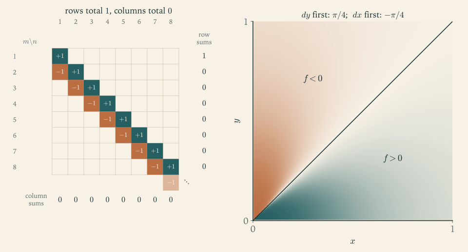
Return to the array of the chapter opening, \(a_{m,n}=1\) if \(m=n\) , \(-1\) if \(m=n+1\) , \(0\) otherwise. It is a function on \(\mathbb N\times\mathbb N\) , and with counting measure on each factor, which is \(\sigma\) -finite, the iterated integrals are iterated sums:
Fubini’s theorem is not contradicted, because its hypothesis fails: there are infinitely many entries of absolute value \(1\) , so
Tonelli’s theorem, applied to \(\lvert a_{m,n}\rvert\) , is what certifies this: the sum of the absolute values is the same in every order, and it is infinite. The left panel of Figure 6.1 shows the array with its row and column sums.
Example 6.4: A rational function with two different iterated integrals
On the open unit square let
Since \(\dfrac{\partial}{\partial y}\dfrac{y}{x^2+y^2}=\dfrac{x^2-y^2}{(x^2+y^2)^2}\) , for each \(x\in(0,1)\)
The function is antisymmetric, \(f(y,x)=-f(x,y)\) , so the other order gives
Both iterated integrals exist, both are finite, and they differ. Therefore \(f\) is not integrable on the square. To see this directly, apply Tonelli to the positive part: \(f\ge0\) on the triangle \(\{0<y<x<1\}\) , and there
The function has a non-integrable singularity at the origin, positive below the diagonal and negative above it, and the two orders of integration cancel the infinities differently. The right panel of Figure 6.1 shows the sign pattern.
Common mistake. Concluding that two iterated integrals are equal because both exist and are finite. Example 6.4 refutes this. Existence of the iterated integrals is a conclusion of Fubini’s theorem, not its hypothesis; the hypothesis is that the absolute value has a finite integral, and that is checked with Tonelli.
Example 6.5: The Gaussian integral
Let \(I=\int_0^\infty e^{-x^2}\,dx\) . Then
For fixed \(x>0\) substitute \(y=xt\) in the inner integral; by Exercise 4.13 a dilation by \(x\) multiplies the integral by \(x\) , so \(\int_0^\infty e^{-y^2}\,dy=x\int_0^\infty e^{-x^2t^2}\,dt\) . Hence
The integrand is nonnegative and continuous on the open quadrant, so Tonelli allows the exchange, and the inner integral in \(x\) is elementary:
Therefore \(I=\dfrac{\sqrt\pi}{2}\approx0.8862\) , and \(\int_{-\infty}^\infty e^{-x^2}\,dx=\sqrt\pi\) . No polar coordinates were needed, only a dilation in one variable and one exchange of order.
Example 6.6: A diagonal that defeats the theorem without sigma-finiteness
Let \(X=Y=[0,1]\) with the Borel sets, let \(\mu=\lambda\) , and let \(\nu\) be counting measure, which is not \(\sigma\) -finite on an uncountable set. The diagonal \(D=\{(x,x):x\in[0,1]\}\) is closed in the plane, hence in \(\mathcal B\otimes\mathcal B\) . Each section \(D_x=\{x\}\) and \(D^y=\{y\}\) is a single point, so
The function \(\mathbf 1_D\) is nonnegative and measurable, and its two iterated integrals disagree. The only hypothesis of Tonelli’s theorem that fails is \(\sigma\) -finiteness of \(\nu\) . In the proof it was needed to reduce to finite measures, where differences of measures of sections make sense.
6.4 Two consequences
Tonelli’s theorem turns the picture of an integral as an area under a graph into an identity, and the identity is the horizontal slicing of Chapter 4 in its final form.
Proposition 6.7 (integration by layers). Let \(\mu\) be \(\sigma\) -finite, let \(f:X\to[0,\infty)\) be measurable, and let \(0<p<\infty\) . Then
In particular \(\int f\,d\mu=\int_0^\infty\mu(\{f>t\})\,dt\) .
Proof. The set \(E=\{(x,t)\in X\times[0,\infty):t<f(x)\}\) belongs to the product \(\sigma\) -algebra, because \((x,t)\mapsto f(x)-t\) is measurable as a difference of measurable functions of the coordinates. Apply Tonelli’s theorem to \(g(x,t)=pt^{p-1}\mathbf 1_E(x,t)\) on \(X\times[0,\infty)\) with the measure \(\mu\times\lambda\) . Integrating first in \(t\) : for fixed \(x\) the section is \([0,f(x))\) and \(\int_0^{f(x)}pt^{p-1}\,dt=f(x)^p\) . Integrating first in \(x\) : for fixed \(t\) the section is \(\{f>t\}\) , giving \(pt^{p-1}\mu(\{f>t\})\) .
The function \(t\mapsto\mu(\{f>t\})\) is the distribution function of \(f\) . The proposition says that the integral of \(f\) , and of every power of \(f\) , depends on \(f\) only through it. For \(p=1\) it says that the region under the graph has product measure \(\int f\,d\mu\) whether it is cut into vertical or horizontal slices.
Example 6.7: A singular integral computed by layers
Let \(f(x)=x^{-1/2}\) on \((0,1)\) with Lebesgue measure. For \(t<1\) every point satisfies \(f(x)>t\) , so \(\lambda(\{f>t\})=1\) . For \(t\ge1\) , \(f(x)>t\) means \(x<t^{-2}\) , so \(\lambda(\{f>t\})=t^{-2}\) . By Proposition 6.7,
in agreement with Example 4.3. With \(p=2\) the formula gives \(\int_0^1f^2\,d\lambda=\int_0^12t\,dt+\int_1^\infty2t\cdot t^{-2}\,dt=1+\infty\) , so \(f^2=x^{-1}\) is not integrable: the distribution function decays like \(t^{-2}\) , which is integrable against \(1\) but not against \(2t\) .
Proposition 6.8 (convolution of integrable functions). Let \(f,g:\mathbb R\to\mathbb R\) be Borel measurable and Lebesgue integrable. Then for almost every \(x\) the function \(y\mapsto f(x-y)g(y)\) is integrable, the convolution
is an integrable function of \(x\) , and \(\int\lvert f*g\rvert\,d\lambda\le\int\lvert f\rvert\,d\lambda\cdot\int\lvert g\rvert\,d\lambda\) .
Proof. The function \(h(x,y)=f(x-y)g(y)\) is Borel measurable on \(\mathbb R^2\) : \((x,y)\mapsto x-y\) and \((x,y)\mapsto y\) are continuous, and compositions and products of Borel functions are Borel. By Tonelli, integrating first in \(x\) and using translation invariance of \(\lambda\) ,
So \(h\) is integrable on the plane, and Fubini’s theorem gives everything claimed: almost every section in \(x\) is integrable, the resulting function of \(x\) is integrable, and \(\int\lvert f*g\rvert\le\int\!\!\int\lvert h\rvert\) .
The proof is the standard pattern in miniature: measurability on the product first, Tonelli on the absolute value second, Fubini third.
With products in hand, integrals over \(\mathbb R^d\) are available. The next question is about the functions themselves. The integrable functions form a vector space with a natural notion of size, \(\int\lvert f\rvert\,d\mu\) . Is that a norm, what are its relatives for other powers, and how do they control products and sums?
Exercises
-
With \(X\) , \(Y\) , \(\mu\) , \(\nu\) as in Example 6.1, let \(F=(\{2,3\}\times\{1,2\})\cup(\{1\}\times\{1\})\) . List the sections \(F_x\) and \(F^y\) and compute \((\mu\times\nu)(F)\) by both slicings.
Answer
\(F_1=\{1\}\) and \(F_2=F_3=\{1,2\}\) ; \(F^1=\{1,2,3\}\) and \(F^2=\{2,3\}\) . Slicing by \(x\) : \(\int\nu(F_x)\,d\mu=1\cdot2+2\cdot3=8\) . Slicing by \(y\) : \(\int\mu(F^y)\,d\nu=5+3=8\) . So \((\mu\times\nu)(F)=8\) .
-
Evaluate \(\displaystyle\int_0^1\Bigl(\int_y^1\frac{\sin x}{x}\,dx\Bigr)dy\) by reversing the order of integration, stating which theorem applies and why its hypothesis holds.
Solution
The inner integral cannot be evaluated in closed form, so reverse the order. The integrand is \(h(x,y)=\dfrac{\sin x}{x}\mathbf 1_{\{0<y<x<1\}}\) , a continuous function times the indicator of an open triangle, hence Borel measurable on the plane. It satisfies \(\lvert h\rvert\le1\) on the unit square, which has finite measure, so \(\int\lvert h\rvert\,d(\lambda\times\lambda)\le1<\infty\) and Fubini’s theorem applies. (Since \(\sin x>0\) on \((0,1)\) the integrand is in fact nonnegative and Tonelli’s theorem would do.) For fixed \(x\) the variable \(y\) runs over \((0,x)\) :
\[ \int_0^1\Bigl(\int_y^1\frac{\sin x}{x}\,dx\Bigr)dy=\int_0^1\Bigl(\int_0^x\frac{\sin x}{x}\,dy\Bigr)dx=\int_0^1\frac{\sin x}{x}\cdot x\,dx=\int_0^1\sin x\,dx=1-\cos1\approx0.4597 . \]The factor \(x\) produced by the inner integration cancels the denominator, which is why this order is the tractable one.
-
For \(0<a<b\) show that \(\dfrac{x^b-x^a}{\ln x}=\displaystyle\int_a^bx^t\,dt\) for \(0<x<1\) , and use Tonelli’s theorem to evaluate \(\displaystyle\int_0^1\frac{x^b-x^a}{\ln x}\,dx\) ; give the value for \(a=1\) , \(b=3\) .
Solution
For \(0<x<1\) and real \(t\) , \(x^t=e^{t\ln x}\) , so \(\int_a^bx^t\,dt=\Bigl[\dfrac{x^t}{\ln x}\Bigr]_{t=a}^{t=b}=\dfrac{x^b-x^a}{\ln x}\) . Both numerator and denominator are negative, so the quotient is positive, as an integral of the positive function \(x^t\) must be.
The function \((x,t)\mapsto x^t\) is continuous and nonnegative on \((0,1)\times(a,b)\) . By Tonelli’s theorem,
\[ \int_0^1\frac{x^b-x^a}{\ln x}\,dx=\int_0^1\Bigl(\int_a^bx^t\,dt\Bigr)dx=\int_a^b\Bigl(\int_0^1x^t\,dx\Bigr)dt=\int_a^b\frac{dt}{t+1}=\ln\frac{b+1}{a+1}. \]For \(a=1\) and \(b=3\) the value is \(\ln\frac42=\ln2\approx0.6931\) . No estimate was required because the integrand of the double integral is nonnegative; the original single integral, by contrast, has an integrand with an apparent singularity at \(x=1\) that the double-integral representation makes harmless.
-
Let \(\zeta(s)=\sum_{k\ge1}k^{-s}\) . Use Tonelli’s theorem for counting measure to prove that \(\sum_{s=2}^\infty(\zeta(s)-1)=1\) .
Solution
By definition \(\zeta(s)-1=\sum_{k\ge2}k^{-s}\) . The terms \(k^{-s}\) , for integers \(k\ge2\) and \(s\ge2\) , are nonnegative, so by Tonelli’s theorem for counting measure on each index set (equivalently, the double-series form of Theorem 4.5 from Exercise 4.2) the order of summation may be exchanged:
\[ \sum_{s=2}^\infty(\zeta(s)-1)=\sum_{s=2}^\infty\sum_{k=2}^\infty k^{-s}=\sum_{k=2}^\infty\sum_{s=2}^\infty k^{-s}. \]For fixed \(k\ge2\) the inner sum is geometric with ratio \(\tfrac1k\) :
\[ \sum_{s=2}^\infty k^{-s}=\frac{k^{-2}}{1-k^{-1}}=\frac1{k(k-1)}=\frac1{k-1}-\frac1k . \]The outer sum telescopes: \(\sum_{k=2}^\infty\bigl(\frac1{k-1}-\frac1k\bigr)=1\) . Hence \(\sum_{s=2}^\infty(\zeta(s)-1)=1\) . The individual values \(\zeta(s)\) have no simple form for odd \(s\) , yet the exchange of order evaluates the total exactly.
-
A student claims: “Both iterated integrals of \(f\) over the unit square exist and are finite, so by Fubini’s theorem they are equal.” Name a function for which this fails and state the hypothesis that the student did not verify.
Answer
The function of Example 6.4, \(f(x,y)=\frac{x^2-y^2}{(x^2+y^2)^2}\) , has iterated integrals \(\tfrac\pi4\) and \(-\tfrac\pi4\) . The unverified hypothesis is integrability on the product: \(\int\lvert f\rvert\,d(\lambda\times\lambda)<\infty\) , which is to be checked with Tonelli’s theorem and here fails.
-
Let \(b_{m,n}=2^{-m}a_{m,n}\) , where \(a_{m,n}\) is the array of Example 6.3. Show that \(\sum_{m,n}\lvert b_{m,n}\rvert<\infty\) and compute both iterated sums.
Answer
Row \(1\) has the single nonzero entry \(\tfrac12\) and row \(m\ge2\) has the two entries \(\pm2^{-m}\) , so \(\sum_{m,n}\lvert b_{m,n}\rvert=\tfrac12+2\sum_{m\ge2}2^{-m}=\tfrac32<\infty\) . Row sums: \(\tfrac12,0,0,\dots\) , total \(\tfrac12\) . Column \(n\) has entries \(2^{-n}\) and \(-2^{-n-1}\) , sum \(2^{-n-1}\) ; total \(\sum_n2^{-n-1}=\tfrac12\) . The two orders agree, as Fubini’s theorem requires.
-
Let \(f:\mathbb R\to\mathbb R\) be Borel measurable. Prove that its graph \(\{(x,f(x)):x\in\mathbb R\}\) is a Borel subset of the plane with \((\lambda\times\lambda)\) -measure zero.
Solution
The graph is Borel. The function \(h(x,y)=f(x)-y\) is Borel measurable on \(\mathbb R^2\) : \((x,y)\mapsto f(x)\) is the composition of the continuous projection with the Borel function \(f\) , and \((x,y)\mapsto y\) is continuous. The graph is \(G=h^{-1}(\{0\})\) , the preimage of a closed set, so \(G\in\mathcal B(\mathbb R^2)=\mathcal B(\mathbb R)\otimes\mathcal B(\mathbb R)\) .
It has measure zero. For each \(x\) the section \(G_x=\{y:y=f(x)\}=\{f(x)\}\) is a single point, so \(\lambda(G_x)=0\) . Lebesgue measure is \(\sigma\) -finite, and Theorem 6.4 gives
\[ (\lambda\times\lambda)(G)=\int_{\mathbb R}\lambda(G_x)\,d\lambda(x)=\int_{\mathbb R}0\,d\lambda=0 . \]Notice that the horizontal sections \(G^y=f^{-1}(\{y\})\) can be large: for a constant function one of them is all of \(\mathbb R\) . Theorem 6.4 then forces \(\lambda(G^y)=0\) for almost every \(y\) . That is consistent: the level sets \(f^{-1}(\{y\})\) are pairwise disjoint, so by Exercise 1.14 at most countably many of them have positive measure, and a countable set of heights is null.
-
Let \(\mu,\nu\) be \(\sigma\) -finite and \(E\in\mathcal A\otimes\mathcal B\) with \(\nu(E_x)=0\) for \(\mu\) -almost every \(x\) . Prove that \(\mu(E^y)=0\) for \(\nu\) -almost every \(y\) .
Solution
By Theorem 6.4 the functions \(x\mapsto\nu(E_x)\) and \(y\mapsto\mu(E^y)\) are measurable and nonnegative, and
\[ \int_Y\mu(E^y)\,d\nu(y)=\int_X\nu(E_x)\,d\mu(x). \]The right side is the integral of a nonnegative function that vanishes \(\mu\) -almost everywhere, so it is \(0\) by Proposition 4.7(b). Hence the left side is \(0\) , and it is the integral of the nonnegative measurable function \(y\mapsto\mu(E^y)\) . Applying Proposition 4.7(b) in the other direction, that function vanishes \(\nu\) -almost everywhere. In words: a set in a product is null if almost all of its vertical sections are null, and then almost all of its horizontal sections are null too. Both hypotheses of \(\sigma\) -finiteness were used, through Theorem 6.4; The diagonal of Example 6.6 shows that the statement is false without them: take \(\mu\) to be counting measure and \(\nu\) Lebesgue measure on \([0,1]\) . Every section \(D_x\) is a single point, which is \(\nu\) -null, yet \(\mu(D^y)=1\) for every \(y\) .
-
Use Theorem 6.4 to compute the area \((\lambda\times\lambda)(\{(x,y):x^2+y^2<1\})\) from the lengths of the vertical sections, and say why the set is in the product \(\sigma\) -algebra.
Answer
The disc is open, hence a Borel subset of the plane, and \(\mathcal B(\mathbb R^2)=\mathcal B(\mathbb R)\otimes\mathcal B(\mathbb R)\) . Its section at \(x\in(-1,1)\) is an interval of length \(2\sqrt{1-x^2}\) , and it is empty otherwise. So the area is \(\int_{-1}^12\sqrt{1-x^2}\,dx=\pi\) .
-
Let \(f:X\to\{0,1,2,\dots\}\) be measurable. Prove that \(\int f\,d\mu=\sum_{k=1}^\infty\mu(\{f\ge k\})\) , and verify it for \(f(j)=j\) on \(\{0,1,2,\dots\}\) with weights \(w(j)=2^{-j-1}\) .
Solution
For a function with values in the nonnegative integers,
\[ f=\sum_{k=1}^\infty\mathbf 1_{\{f\ge k\}} \]at every point: if \(f(x)=j\) , exactly the terms with \(k\le j\) equal \(1\) . The sets \(\{f\ge k\}\) are measurable, and the series has nonnegative terms, so Theorem 4.5 gives \(\int f\,d\mu=\sum_{k\ge1}\mu(\{f\ge k\})\) . This is Proposition 6.7 with \(p=1\) , since \(\mu(\{f>t\})=\mu(\{f\ge k\})\) for \(k-1\le t<k\) , but it needs neither \(\sigma\) -finiteness nor a product measure.
For the weights \(w(j)=2^{-j-1}\) on \(\{0,1,2,\dots\}\) and \(f(j)=j\) ,
\[ \mu(\{f\ge k\})=\sum_{j\ge k}2^{-j-1}=2^{-k},\qquad\sum_{k=1}^\infty2^{-k}=1 . \]Directly, \(\int f\,d\mu=\sum_{j\ge0}j\,2^{-j-1}=\tfrac12\sum_{j\ge1}j2^{-j}=\tfrac12\cdot2=1\) , using the sum from Example 4.2. The two computations agree, and the first one needed only a geometric series.
-
Compute the convolution \(\mathbf 1_{[0,1]}*\mathbf 1_{[0,1]}\) explicitly, sketch it, and verify that its integral equals the product of the integrals of the two factors.
Solution
Let \(f=g=\mathbf 1_{[0,1]}\) . Then \(f(x-y)g(y)=1\) exactly when \(0\le y\le1\) and \(x-1\le y\le x\) , so
\[ (f*g)(x)=\lambda\bigl([0,1]\cap[x-1,x]\bigr). \]The two intervals are disjoint if \(x<0\) or \(x>2\) . For \(0\le x\le1\) the intersection is \([0,x]\) , of length \(x\) . For \(1\le x\le2\) it is \([x-1,1]\) , of length \(2-x\) . Hence
\[ (f*g)(x)=\begin{cases}x,&0\le x\le1,\\ 2-x,&1\le x\le2,\\ 0,&\text{otherwise},\end{cases} \]a tent of height \(1\) over the base \([0,2]\) . Its integral is the area of a triangle with base \(2\) and height \(1\) , namely \(1\) , which equals \(\int f\,d\lambda\cdot\int g\,d\lambda=1\cdot1\) . For nonnegative functions the inequality of Proposition 6.8 is an equality, by Tonelli’s theorem. The convolution of two discontinuous functions has come out continuous, a first instance of the smoothing effect that Chapter 8 exploits.
-
Let \(f(x,y)=\dfrac{xy}{(x^2+y^2)^2}\) on \([-1,1]^2\) , with \(f(0,0)=0\) . Show that both iterated integrals exist and equal \(0\) , and that \(f\) is nevertheless not integrable on the square.
Hint
For fixed \(y\ne0\) the function \(x\mapsto f(x,y)\) is continuous and odd on \([-1,1]\) , so its integral is \(0\) ; for \(y=0\) it vanishes identically. For non-integrability restrict to \((0,1)^2\) , where \(f>0\) , and compute \(\int_0^1f(x,y)\,dx=\frac1{2y}-\frac{y}{2(1+y^2)}\) , which is not integrable in \(y\) near \(0\) .
-
Starting from \(\dfrac1x=\displaystyle\int_0^\infty e^{-xt}\,dt\) , apply Fubini’s theorem on \((0,T)\times(0,\infty)\) and then dominated convergence as \(T\to\infty\) to prove that \(\displaystyle\lim_{T\to\infty}\int_0^T\frac{\sin x}{x}\,dx=\frac\pi2\) .
Hint
On \((0,T)\times(0,\infty)\) , \(\int\!\!\int\lvert e^{-xt}\sin x\rvert\,dt\,dx=\int_0^T\frac{\lvert\sin x\rvert}{x}\,dx\le T\) , so Fubini applies and \(\int_0^T\frac{\sin x}x\,dx=\int_0^\infty\bigl(\int_0^Te^{-xt}\sin x\,dx\bigr)dt\) . The inner integral is \(\dfrac{1-e^{-tT}(\cos T+t\sin T)}{1+t^2}\) . For \(T\ge1\) it is bounded by \(\dfrac{1+(1+t)e^{-t}}{1+t^2}\) , which is integrable, and it tends to \(\dfrac1{1+t^2}\) .
-
Prove that \(\mathcal P(\mathbb N)\otimes\mathcal P(\mathbb N)=\mathcal P(\mathbb N\times\mathbb N)\) and that the product of counting measure with itself is counting measure on \(\mathbb N\times\mathbb N\) .
Hint
Every singleton \(\{(m,n)\}=\{m\}\times\{n\}\) is a rectangle, and every subset of the countable set \(\mathbb N\times\mathbb N\) is a countable union of singletons. For the measure, check the rectangle formula on singletons and use uniqueness in Theorem 6.4.
-
Let \(\mu,\nu\) be finite Borel measures on \([a,b]\) without atoms, so that the distribution functions \(F(x)=\mu([a,x])\) and \(G(x)=\nu([a,x])\) are continuous with \(F(a)=G(a)=0\) . By computing \((\mu\times\nu)\) of the square in two ways, prove \(\int F\,d\nu+\int G\,d\mu=F(b)G(b)\) , and say what must be added to the right side when both measures have an atom at \(a\) .
Hint
The square \([a,b]^2\) has product measure \(F(b)G(b)\) . Split it into \(\{x\le y\}\) and \(\{x>y\}\) . By Theorem 6.4 the first has measure \(\int\mu([a,y])\,d\nu(y)=\int F\,d\nu\) , and the second has measure \(\int\nu([a,x))\,d\mu(x)\) , which equals \(\int G\,d\mu\) because \(\nu\) has no atoms. Without that assumption the second region contributes \(\int G(x^-)\,d\mu(x)\) ; if the only common atom is at \(a\) , the correction is the term \(\mu(\{a\})\nu(\{a\})\) added to \(F(b)G(b)\) , as the measures \(\mu=\nu=\delta_a\) show, with left side \(2\) and \(F(b)G(b)=1\) .
-
Compute both iterated integrals of \(f(x,y)=\dfrac{x-y}{(x+y)^3}\) over the open unit square, and decide whether \(f\) is integrable there.
Solution
Since \(\dfrac{\partial}{\partial y}\dfrac{y}{(x+y)^2}=\dfrac{(x+y)-2y}{(x+y)^3}=\dfrac{x-y}{(x+y)^3}\) , for each \(x\in(0,1)\)
\[ \int_0^1\frac{x-y}{(x+y)^3}\,dy=\Bigl[\frac{y}{(x+y)^2}\Bigr]_{y=0}^{y=1}=\frac1{(1+x)^2},\qquad\int_0^1\frac{dx}{(1+x)^2}=\frac12 . \]The function is antisymmetric under exchanging \(x\) and \(y\) , so the other order gives \(-\tfrac12\) :
\[ \int_0^1\Bigl(\int_0^1f\,dy\Bigr)dx=\frac12,\qquad\int_0^1\Bigl(\int_0^1f\,dx\Bigr)dy=-\frac12 . \]The two iterated integrals differ, so by Fubini’s theorem \(f\) cannot be integrable on the square. Directly: \(f\ge0\) on \(\{0<y<x\}\) , where \(\int_0^xf\,dy=\frac{x}{(2x)^2}=\frac1{4x}\) , and \(\int_0^1\frac{dx}{4x}=\infty\) ; by Tonelli \(\int f^+\,d(\lambda\times\lambda)=\infty\) . The singularity at the origin is of order \(r^{-2}\) in the distance \(r\) , which is exactly the borderline of integrability in the plane.
-
Let \(f\in L^1(\mu)\) and \(g\in L^1(\nu)\) with \(\mu,\nu\) \(\sigma\) -finite. Prove that \(h(x,y)=f(x)g(y)\) is integrable for \(\mu\times\nu\) and that \(\int h\,d(\mu\times\nu)=\int f\,d\mu\cdot\int g\,d\nu\) .
Hint
The function \(h\) is measurable as a product of functions of the two coordinates. By Tonelli, \(\int\lvert h\rvert\,d(\mu\times\nu)=\int\lvert f\rvert\,d\mu\cdot\int\lvert g\rvert\,d\nu<\infty\) . Then apply Fubini and take the constant \(f(x)\) out of the inner integral.